Data Analysis

Welcome to the Data Analysis module on the Chisquares platform—the epicenter of insight generation and decision support. Whether you’re a researcher, business analyst, or healthcare professional, this module transforms raw survey responses into clear, actionable intelligence with just a few clicks. With Chisquares’ Data Analysis module, you’re not just crunching numbers—you’re unlocking the story behind your data. Dive in, explore, and let your insights lead the way.

Imagine:

1. Instantly uploading your dataset and seeing its structure come to life in the Dataset Codebook.
2. Effortlessly applying filters, recoding variables, or creating composites via the quick-access menus.
3. One-click generation of tables, charts, and regression models—then pushing them directly into your manuscript or report.

Why You’ll Love It

• Speed & Simplicity
  No more wrestling with spreadsheets or writing custom code. An intuitive, point-and-click interface guides you from data import to final report.

• Complete Control
  From variable-level edits (e.g., rename, recode, split, clone) to dataset-wide actions (e.g., weight calibration), every transformation is reversible and non-destructive.

• AI-Driven Guidance
  Let the Analysis Wizard suggest the most appropriate tests, highlight outliers, and even propose research questions—so you can focus on interpretation, not setup.

• Publication-Ready Outputs
  Generate polished tables and figures (histograms, boxplots, contingency tables, regression diagnostics) in seconds, exportable as CSV, PDF, PNG—and insertable directly into your documents.

Core Features

1. Data Processing & Analysis

• Upload survey data (CSV, Excel, built-in surveys, public repositories).
• Transform variables: numeric adjustments, date extractions, visual or rule-based recodes, composite generation.
• Explore with built-in descriptive stats and frequency summaries.

2. Search, Filter & Sort

• Search Bar – Find any analysis by name or keyword.
• Filter – Drill down by date, user, dataset attributes, or custom criteria.
• Sort – Order your projects by recency, relevance, or custom tags.

3. Automated Insights & Reporting

• AI Suggestions – Smart recommendations for tables, charts, and regression models.
• Outlier Detection – Flag unexpected values and distributional shifts automatically.
• Export & Reporting – Compile summary reports with a single click, in CSV, PDF, or ready-to-publish formats.

Getting Started

To use the Data Analysis module effectively, follow these simple steps:

1. Accessing Data Analysis Module

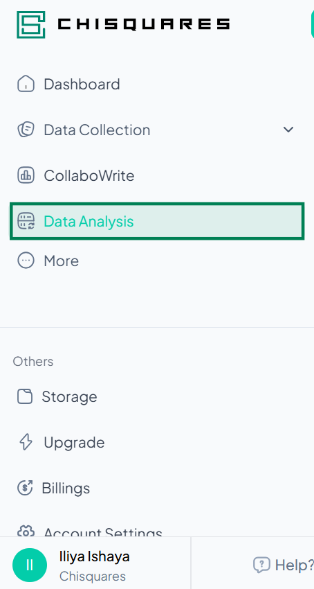
• Log in to your Chisquares account.
• In the left-hand navigation bar, select Data Analysis.

2. Launching the Data Analysis Section

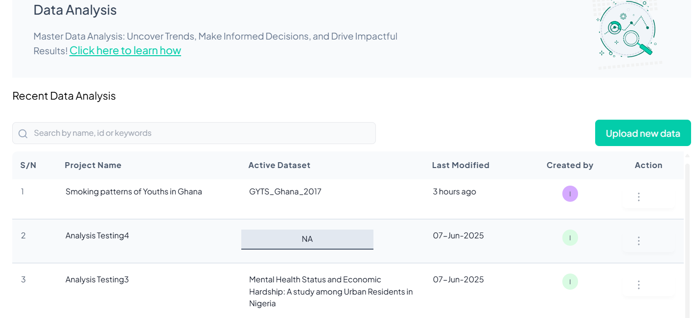
Once you click Data Analysis, you will be taken to the Data Analysis page.

Features on This Page:

• Intro text and onboarding link.
• A searchable list of recent analyses.
• A prominent Upload new data button

3. Creating a New Analysis Project

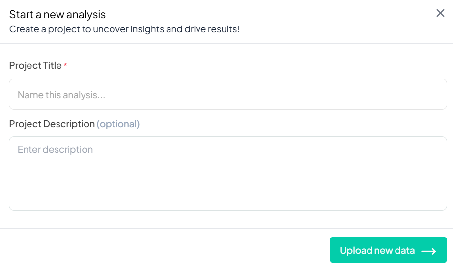
Click the Upload new data button to create a new project.

Required Inputs:

• Project Title (mandatory)
• Project Description (optional)

After filling in the details, click Upload new data to proceed.

Importing and Managing Datasets

Who Can Upload or View Datasets?

• All collaborators in a project can upload and view datasets

Only Project Owners can delete datasets

What Can You Import?

Chisquares supports the import of:

• CSV (.csv)

• Excel (.xls, .xlsx)

• Public datasets (cleaned and curated)

• Survey data collected using the platform itself

Each uploaded dataset becomes part of the current project and can be used for immediate analysis.

When to Import a Dataset

Import a dataset when:

• You begin a new analysis

• You want to use public data stored by Chisquares

• You’ve collected survey responses through the platform

• You’re replacing an old dataset with a newer version

Where to import dataset from

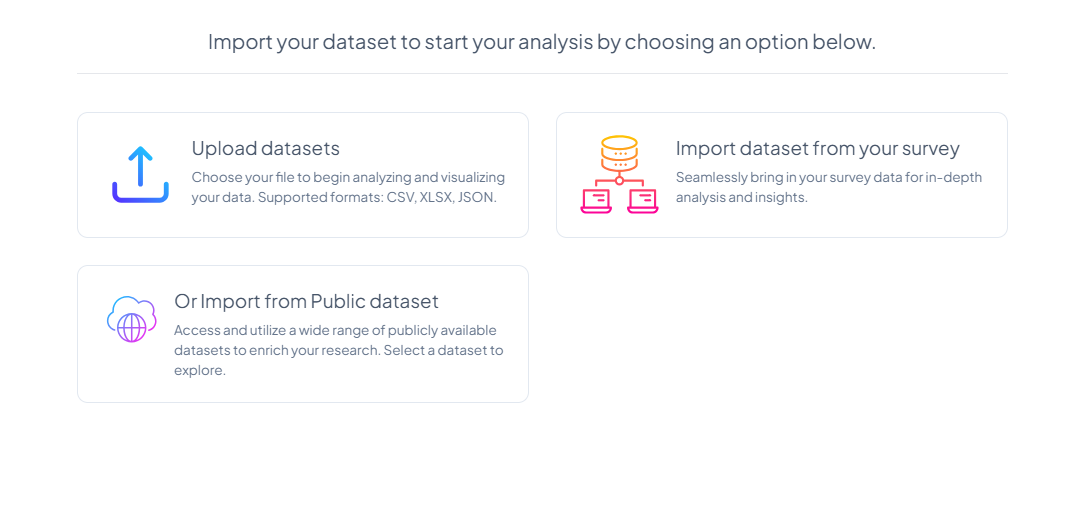
Choose a source:

• Upload datasets

• Import dataset from your survey

• Import from data dataset

Uploading a Dataset

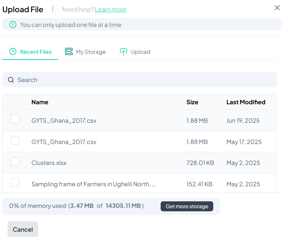
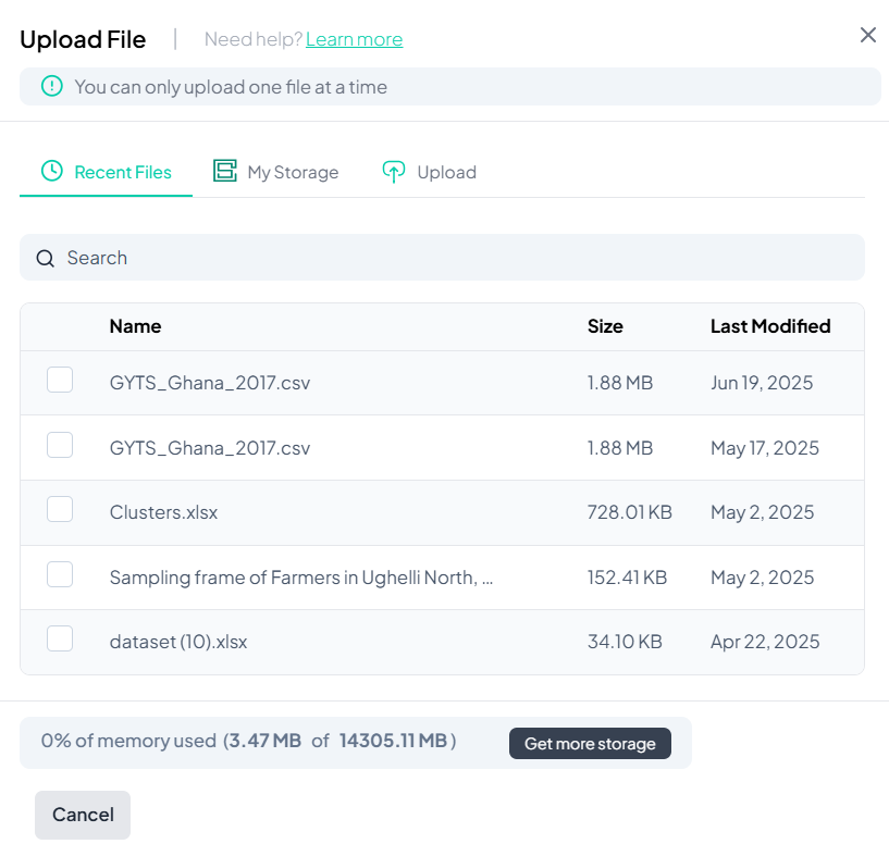
If you select Upload datasets, you’ll see a file picker screen.

• Select from Recent Files, My Storage, or manually Upload
• Click to check the dataset
• Click Import

Viewing and Managing Your Dataset

Once the dataset is imported:

Key Elements on Screen:

• Dataset information (ID, source, import date, etc.)
• List of variables and their types
• Buttons for Data Processing, Estimate, Test, and Analysis Wizard.
• Prompt to enable Weighted Analysis (optional)

Click Yes to set weights if needed, or No to proceed unweighted.

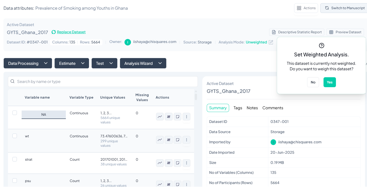
Verify Dataset Information

• Check the Dataset ID and Name at the top left to ensure you're working on the correct dataset.
• Review the Owner and Import Metadata:
  • Imported by: Confirms who uploaded the dataset.
  • Date Imported: Date when data was uploaded.
  • Number of Variables (Columns) and Participants (Rows): Gives a quick overview of dataset size.

Use the Codebook Panel

Click the Codebook panel (top right) to:

• View detailed metadata of the selected variable.
• See its distribution and value labels (for categorical).
• Check if the variable has missing values or notes.

Use this before proceeding with analysis to understand your data.

Exploring the Dataset Codebook

What Is the Codebook?

The Dataset Codebook is your control panel for understanding and managing variables in your uploaded dataset. It provides a live overview of your dataset’s structure and offers quick access to variable-specific actions like renaming, recoding, visualization, and more.

When Do You Use It?

Immediately after uploading a dataset or whenever you want to:

• Review dataset structure
• Check for missing data
• Perform basic descriptive stats
• Rename, recode, or manage variable types

Where to Find It

Once a dataset is uploaded, Chisquares automatically redirects you to the Dataset Codebook page.

How to Use the Codebook

1. View Dataset Overview

   • Dataset label and actual file name
   • Import date and user
   • Size: number of rows (observations) and columns (variables)
   • Number of missing data

2. Access both Dataset and Variable View

   • Check the box beside the entire dataset, or beside the specific variable you wish to view its attributes.
   • Dataset Attributes (summary of all variables)
   • Variable Attributes (details of selected variable)

3. Explore Variables

   • Click on any variable to see:
     • Five-number summary (for numeric variables)
     • Frequencies (for categorical variables)
     • Unique values and missing counts

4. Edit or Transform Variables
   Next to each variable, you can:

   • Rename or Relabel
   • Recode values
   • Respecify Type (e.g., from integer to categorical)
   • Clone a variable
   • Delete (with recovery option)
   • Visualize: plot a graph for the variable
   • Cross-tabulate with another categorical variable

5. Add Notes and Tags
   Tagging helps organize variables:

   • Add project-specific notes
   • Use searchable tags for easier variable management

6. Review Analysis History
   Track all actions taken on the dataset:

   • Transformations
   • Analyses
   • Recode operations

7. Monitor Dataset Modifications
   A “Last Modified” tag at the top shows the date and time of the most recent change.

Who Can Use the Codebook?

• All collaborators can view and interact with the codebook
• Only users with edit privileges can modify variable settings or delete variables

Why Use the Codebook?

• Gain rapid insight into your dataset’s health and readiness
• Efficiently prepare data for analysis
• Collaborate seamlessly with full traceability of changes

Working with Variables

Variable Classification Guide

The Chisquares platform employs an interpreted framework to classify variables into types such as Continuous, Counts, Binary, Categorical, and others, rather than a strictly statistical approach. This classification determines the available analysis options for each variable. If the platform's auto-classification is incorrect, use the Respecify option to adjust it manually. Below is an overview of the classification types and reclassification options.

Classification Options

Continuous Variables

• Definition: Variables with a theoretically infinite number of unique numeric values.

• Practical Threshold: The system sets a threshold for the number of unique numeric values to approximate infinity.

• Additional Criteria: Variables with decimal places (floats) are classified as Continuous, even if they do not meet the unique value threshold.

• Example: Values such as 3.14, 5.67, or 9.001.

Count Variables

• Definition: Integers with a finite number of unique, non-negative values (zero or greater) below the infinity threshold.

• Key Restriction: Cannot include negative values.

• Example: Values such as 0, 5, or 10 possibly representing counts of occurrences.

Discrete Variables

• Definition: Integers with a finite number of unique values below the infinity threshold, which may include both positive and negative values or only negative values.

• Example: Values such as -5, 0, or 7.

Binary Variables

• Definition: Dichotomous variables coded strictly as 0 and 1. The count of unique values excludes missing values.

• Note: Other dichotomous variables with two unique values (e.g., Yes/No) are classified as Categorical unless coded as 0 and 1.

• Example: Values such as 0 (no) or 1 (yes).

Categorical Variables

• Definition: Variables with categories represented by standardized, repeated alphanumeric characters.

• Example: Values such as Male, Female, or Other.

String Variables

• Definition: Variables with an apparent open-ended set of responses that appear non-standardized or non-repetitive across responses (i.e., high degree of uniqueness).

• Example: Free-text responses such as user comments or descriptions.

Reclassification Options

When using the Respecify option, the platform provides additional granularity for reclassifying variables, particularly for categorical variables, to account for user-specific context:

Nominal Variables

• Definition: Categorical variables with no inherent order among their groups.

• Example: Categories such as Red, Blue, or Green with no ranking.

Ordinal Variables

• Definition: Categorical variables with an inherent order, either ascending or descending.

• Example: Categories such as Low, Medium, or High with a clear ranking.

Key Notes

• The classification of a variable directly impacts the analysis options available on the Chisquares platform.

• Use the Respecify option to correct any misclassifications and ensure the variable type aligns with your analysis needs.

• The system will only allow you to Respecify to options that are statistically plausible. You cannot switch from a string variable to a continuous variable for example.

Visualizing Variables and Creating Charts

What Is Visualization in Chisquares?

Visualization lets you convert variable distributions into clear, customizable graphics. It helps explore data trends, identify outliers, and generate publication-ready figures.

When to Visualize Variables

Use visualization to:

• Understand variable distributions
• Compare groups and categories
• Create manuscript-ready figures
• Explore relationships between variables

Where to Find It

You can visualize any variable by:

1. Going to the Dataset Codebook or Variable Navigation Bar
2. Clicking the visualize icon next to a variable
3. Once the visualization is shown, you can change the type into any of the alternatives shown

How Visualization Works

1. Default Visualization

• When you click “Visualize,” Chisquares creates a basic histogram by default.
• Missing values are excluded.
• Visualization is done with unweighted data.

Why Visualize?

• Improve understanding of data distribution and spread
• Identify errors or outliers before analysis
• Generate figures for publication or peer review
• Save time on formatting and exporting visuals

What Is Variable Management?

Variable management allows you to refine your dataset by renaming labels, reclassifying types, cleaning values, and performing basic transformations — all without writing code.

When to Use These Tools

Use these features when:

• Preparing your data for analysis
• Cleaning inconsistent or unclear variable names
• Adjusting variable types (e.g., converting integer to categorical, such as a socioeconomic status indicator coded as “1”, “2”, “3” which should be treated as categorical, not numeric)
• Creating working copies or simplified versions of variables

Where to Find These Options

In the Dataset Codebook or Variable Navigation Bar, hover over or click the three-dot icon beside any variable to access the following actions:

Actions Menu → Rename / Recode / Clone / Delete / Respecify Type

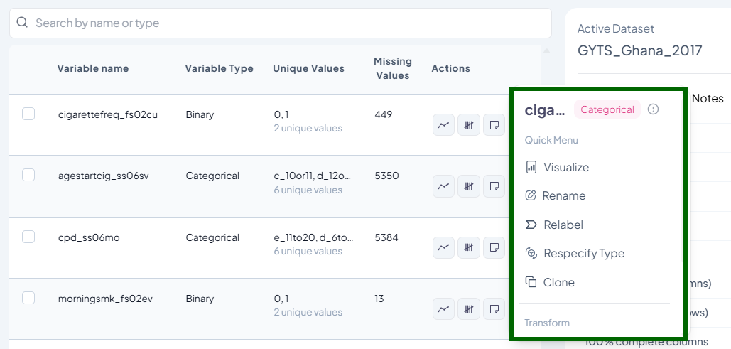
1. Rename Variable Label

   • Purpose: Make variables easier to understand without affecting the original data name.
   • Use Case: Rename “v1_age” to “age_at_enrollment”
   • Steps:
     1. Click the three-dot menu → Rename
     2. Enter a new label (max 20 characters)
     3. Save
   • Validation:
     • Label must be unique
     • Must use letters, numbers, or underscores only

2. Recode Variable Values

   • Purpose: Change values or categories (e.g., merge “Male” and “Other” into one group)
   • Use Case: Combine similar responses into fewer categories
   • Modes:
     • Visual (drag-and-drop interface)
     • Classic (condition-based logic)
   • Features:
     • Create new variable or replace original
     • Treat selected values as missing
     • Recover deleted or merged categories

3. Clone Variable

   • Purpose: Create an exact copy of a variable to test transformations
   • Use Case: Clone “age” as “age_grouped” for categorization
   • Steps:
     1. Click the three-dot menu → Clone
     2. Provide a unique name for the new variable
     3. Save

4. Delete Variable

   • Purpose: Remove an unwanted variable from your dataset
   • Use Case: Remove a variable that was erroneously created to avoid confusion
   • Steps:
     1. Click the three-dot menu → Delete
     2. Confirm deletion
     3. Restore from history using “Recover” option

5. Respecify Variable Type

   • Purpose: Adjust how a variable is treated during analysis (e.g., integer vs. categorical)
   • Use Case: Reclassify a scale score as categorical for group comparisons
   • Steps:
     1. Click the three-dot menu → Respecify Type. You can also reclassify variables from the arrow beside each variable’s classification on the codebook
     2. Select new type (numeric, categorical, date, string)
     3. Confirm
   • Validations:
     • Note that the system automatically ensures that each type switch is compatible with data format.
     • E.g., cannot convert string to numeric unless values are strictly numbers

Why This Matters

Clean, accurate, and well-structured variables:

• Improve analysis quality
• Reduce manual errors
• Enhance collaboration and reproducibility

Data Processing

The Data Processing subsection equips users with tools to prepare and organize their datasets prior to analysis. Operations are grouped into:

• Variable-Level Operations: Manage individual variables (columns).
• Transformations: Apply functional or mathematical changes to variables.
• Dataset-Level Actions: Manage the dataset as a whole.

Each function is non-destructive by default, creating a modified working version without altering the original imported data.

1. Variable-Level Operations

Rename

Within the Data Processing subsection of the Data Analysis module, you can rename one or many variables at once. Follow the steps below to keep your dataset organized and meaningful.

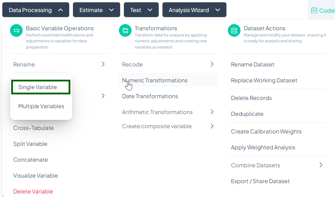
Accessing the Rename Tool

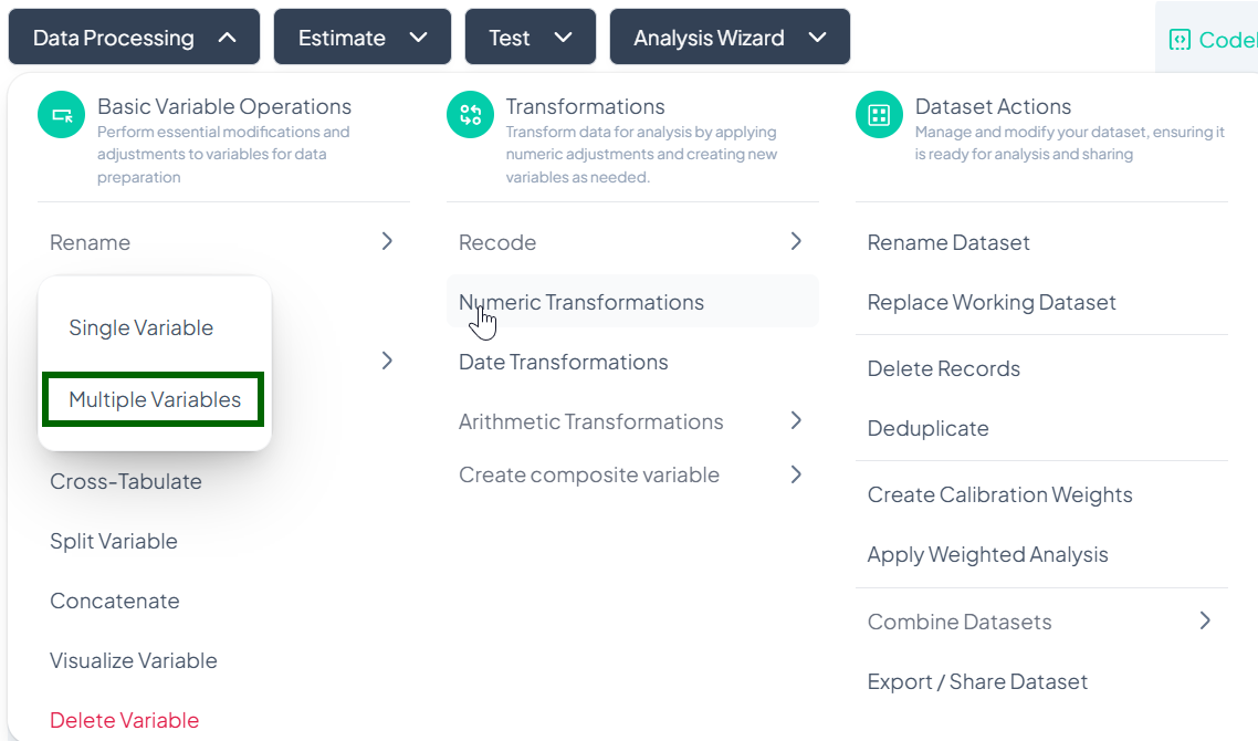
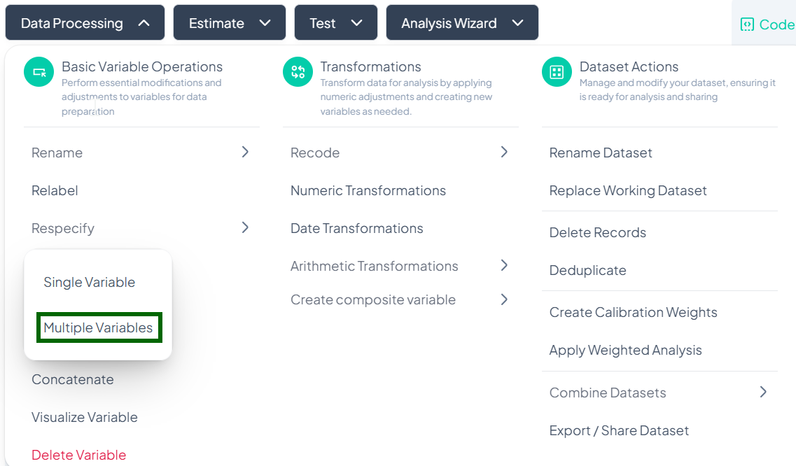
1. Click Data Processing to expand the menu.
2. Under Basic Variable Operations, click Rename.
3. Select Single Variable or Multiple Variables from the pop-out menu.

Single Variable Rename

Use this flow to change the name of one variable at a time.

Step-by-Step Guide

1. Open Single Rename

   • Data Processing → Basic Variable Operations → Rename → Single Variable

   

2. Select Variable

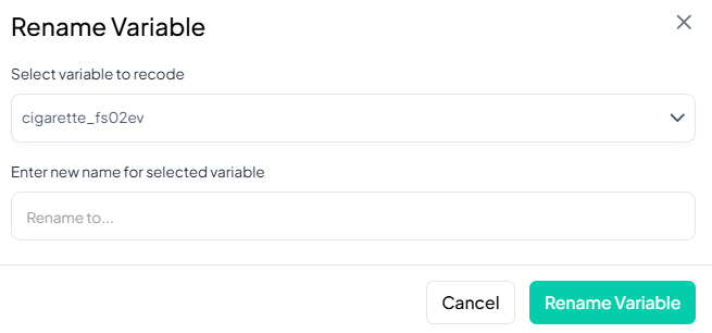
   • In the Rename Variable modal, click the first dropdown and choose the variable you wish to rename.

3. Enter New Name

   • In the “Rename to…” field, type the new variable name.

4. Save

   • Click Rename Variable.
   • The variable’s name updates immediately in your working dataset.

   

Validation Rules

• Unique: New name must not duplicate any existing variable name in the dataset.
• Allowed Characters: A–Z, a–z, 0–9, and underscore ('_') only.
• Length: Maximum of 20 characters.

Multiple Variable Rename

Use this flow to rename several variables at once, saving time when standardizing naming conventions.

Step-by-Step Guide

1. Open Multiple Rename

   • Data Processing → Basic Variable Operations → Rename → Multiple Variables

   

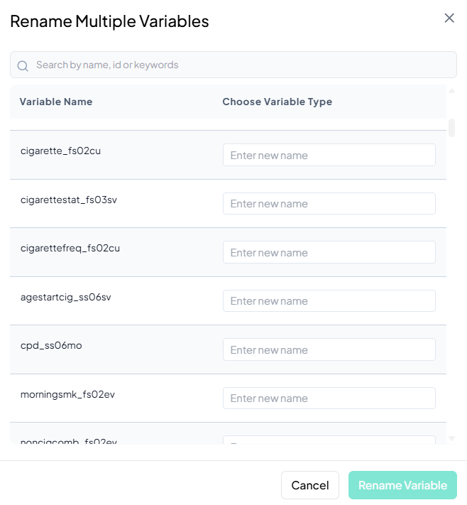
2. Locate Variables

   • In the Rename Multiple Variables modal, scroll or use the search bar to find the variables you want to rename.

3. Enter New Names

   • For each listed variable, click into its Enter new name field and type the desired name.

4. Save

   • Once you’ve renamed all desired variables, click Rename Variable at the bottom of the modal.
   • All changes apply at once to the working dataset.

   

Validation Rules

• Unique: Every new name must be unique across your dataset.
• Allowed Characters: A–Z, a–z, 0–9, and underscore ('_') only.
• Length: Maximum of 20 characters per name.
• Batch Enforcement: If any field fails validation, the Rename Variable button remains disabled until all names comply.

Tip:
If you need to rename dozens of variables following a pattern (e.g. prefixing with 'dem_'), consider renaming in small batches to avoid overwhelming the interface.

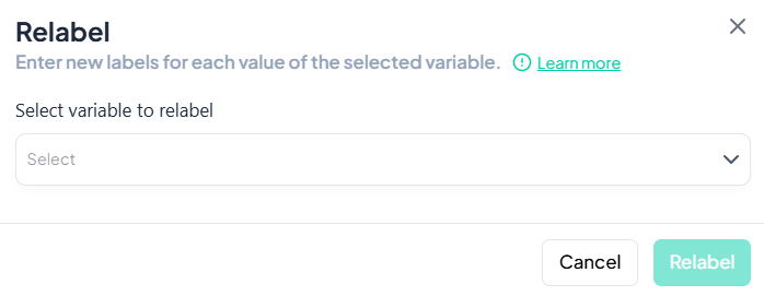
Relabel

Within the Data Processing subsection of the Data Analysis module, you can update the display labels for each value of a variable—without changing the underlying data. Follow the steps below to keep your value labels clear and consistent.

Accessing the Relabel Tool

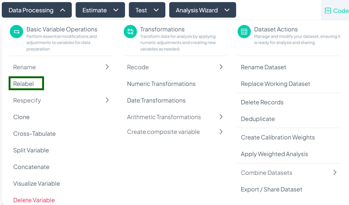
1. Click Data Processing to expand the menu.
2. Under Basic Variable Operations, click Relabel.
3. The Relabel modal will open.

Single Variable Relabel

Use this flow to change the display labels for each value of one variable.

Step-by-Step Guide

1. Open Relabel Modal

   • Data Processing → Basic Variable Operations → Relabel

   

2. Select Variable

   • In the Relabel dialog, click the Select variable to relabel dropdown.
   • Choose the variable whose values you wish to relabel.

3. Enter New Labels

   • A table of all existing values will appear.
   • For each Value, click New Label field and type the desired label.

4. Apply Changes

   • Once all labels are entered, click Relabel.
   • The value labels update immediately in your working dataset.

   

Validation Rules

• Completeness: Every original value must have a non-empty new label before you can proceed.
• Uniqueness: New labels should be distinct to avoid ambiguity in tables and charts.
• Allowed Characters: Letters, numbers, spaces, and punctuation (no control characters).
• Length: While there is no strict character limit, aim for concise, human-readable labels to ensure clarity in outputs.

Tip:
Preview your changes by quickly running a frequency table (via Test → Chi-Square or Estimate → Population Characteristics) to confirm that your new labels display as intended.

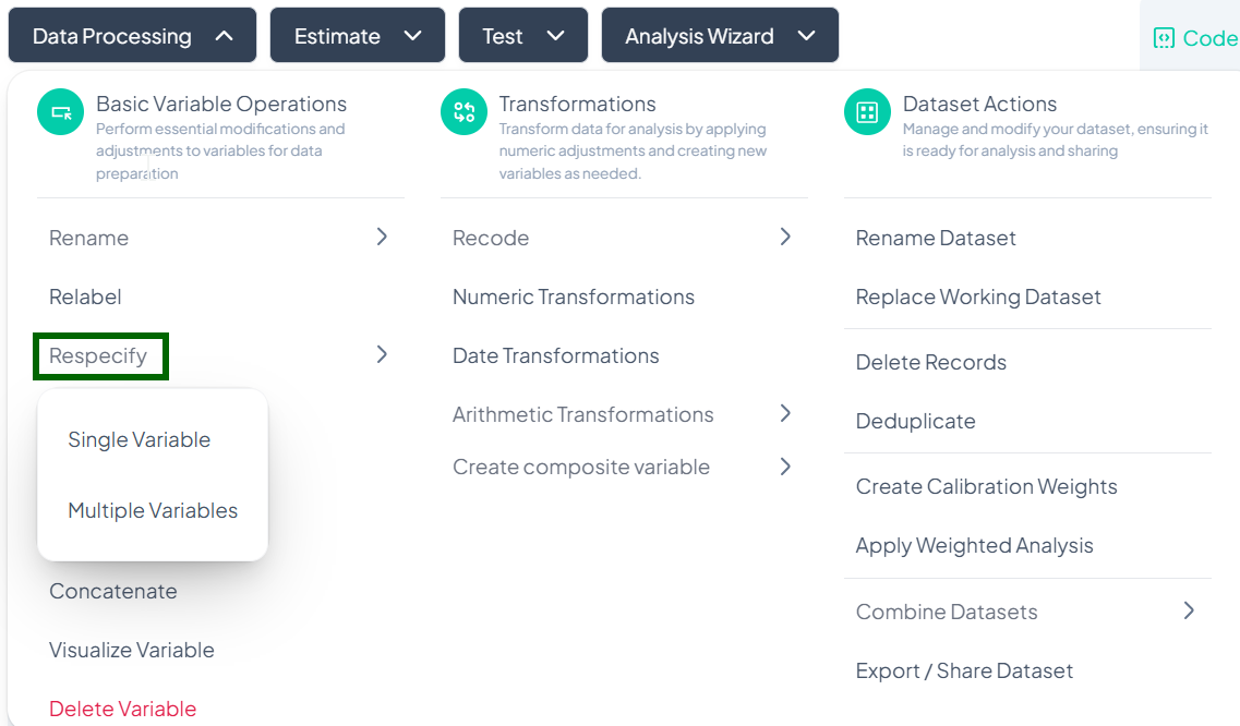
Respecify

Within the Data Processing subsection of the Data Analysis module, the Respecify tool lets you change how variables are classified (e.g., from continuous to categorical) to ensure appropriate analysis methods. Follow the steps below to update one or more variable types without altering the data values.

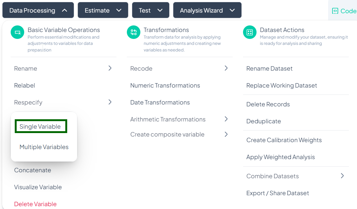
Accessing the Respecify Tool

1. Click Data Processing to expand the menu.
2. Under Basic Variable Operations, click Respecify.
3. Choose Single Variable or Multiple Variables from the pop-out.

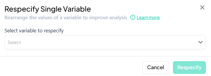
Single-Variable Respecify

Use this flow to change the type classification of one variable (e.g., treating numeric codes as categorical).

Step-by-Step Guide

1. Open Single Respecify

   • Data Processing → Basic Variable Operations → Respecify → Single Variable

   

2. Select Variable

   • In the Select variable to respecify dropdown, choose the target variable.

3. Choose New Type

   • In the modal that appears, select the desired type from options such as:
     • Continuous
     • Count
     • Categorical
     • Binary
     • Date
     • String

4. Confirm

   • Click Respecify.
   • The variable’s type updates immediately, unlocking appropriate analysis tools.

   

Validation Rules

• Compatibility: Only allow conversions that make sense for existing values (e.g., numeric → categorical is allowed; string → continuous only if all values are numeric).
• Immediate Effect: Type change takes effect in the codebook and downstream analysis modules.

Multiple-Variable Respecify

Use this flow to adjust the classifications of several variables at once.

Step-by-Step Guide

1. Open Multiple Respecify

   • Data Processing → Basic Variable Operations → Respecify → Multiple Variables

   

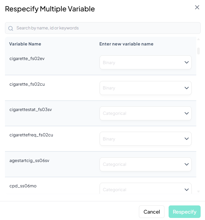
2. Locate Variables

   • In the Respecify Multiple Variable modal, scroll or use the search bar to find each variable you wish to reclassify.

3. Select New Types

   • For each listed variable, click its type dropdown and choose the new classification (Continuous, Count, Categorical, etc.).

4. Confirm

   • Once all selections are made, click Respecify.
   • All chosen variables update in bulk.

   

Validation Rules

• Batch Compatibility: Each selected type must be compatible with the variable’s values.
• All-or-Nothing: The Respecify button remains disabled until every variable has a valid new type chosen.

Tip:
After respecifying, use the Visualize Variable feature to confirm that charts and summaries now display correctly for the new type.

Clone

Within the Data Processing subsection of the Data Analysis module, the Clone tool lets you duplicate an existing variable—preserving its values, labels, and metadata—so you can experiment or transform without affecting the original. Follow the instructions below to clone one variable at a time.

Accessing the Clone Tool

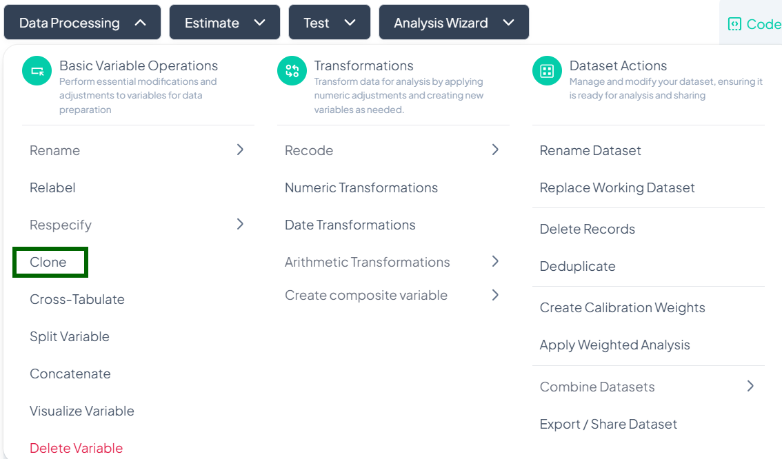
1. Click Data Processing to expand the menu.
2. Under Basic Variable Operations, click Clone.

Cloning a Single Variable

Use this flow to make an exact copy of one variable in your dataset.

Step-by-Step Guide

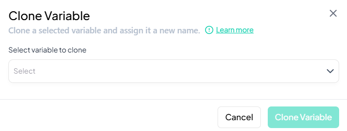
1. Open Clone Modal

   • Data Processing → Basic Variable Operations → Clone

   

2. Select Variable

   • In the Select variable to clone dropdown, choose the variable you want to duplicate.

3. Name the Clone

   • After selecting, an input appears labeled New variable name. Type a unique name for the cloned variable.

4. Confirm

   • Click Clone Variable.
   • A new column is added to your dataset, identical to the original variable.

   

Validation Rules

• Unique Name: The cloned variable’s name must not duplicate any existing variable.
• Metadata Preservation: Value labels, missing codes, and type classifications are copied exactly.

Tip:
Clone a variable before performing irreversible transformations like deletion or recoding, so you always retain the original data.

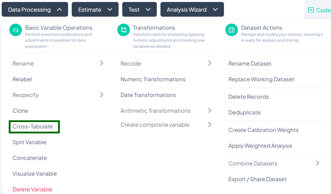
Cross-Tabulate

Within the Data Processing subsection of the Data Analysis module, the Cross-Tabulate tool lets you generate contingency tables for two categorical variables—perfect for exploring relationships between groups. Follow the steps below to create a cross-tabulation.

Accessing the Cross-Tabulate Tool

1. Click Data Processing to expand the menu.
2. Under Basic Variable Operations, click Cross-Tabulate.

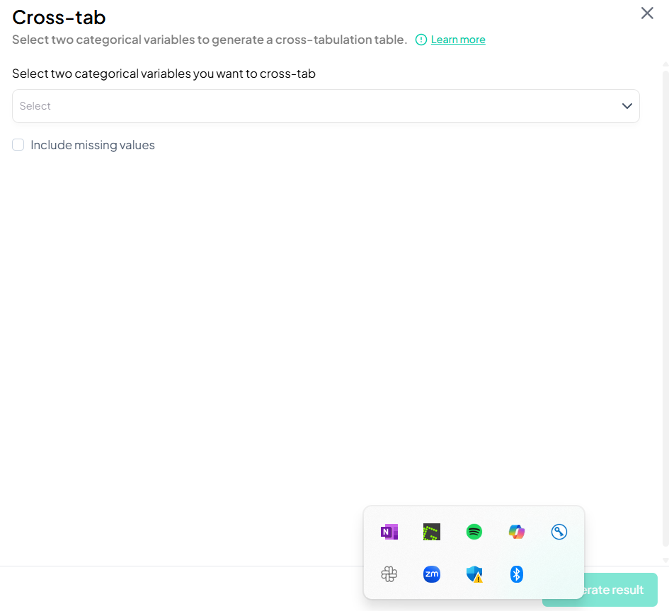
Creating a Cross-Tabulation

Use this flow to select two categorical variables and produce a table showing counts (and optionally percentages) at each combination of levels.

Step-by-Step Guide

1. Open Cross-Tabulate Modal

   • Data Processing → Basic Variable Operations → Cross-Tabulate

   

2. Select Variables

   • In the Select two categorical variables you want to cross-tab dropdown, click to choose both variables (e.g., gender, 'smoker_status').

3. Include Missing Values (Optional)

   • Check Include missing values if you want to count and display missing categories.

4. Generate Table

   • Click Generate result.
   • The cross-tabulation appears inline or in a new tab, showing cell counts and row/column percentages if enabled.

   

Validation Rules

• Variable Types: Only variables classified as categorical (including binary) are available.
• Two Variables: Exactly two variables must be selected.
• Unique Names: Variable names must be distinct; the tool prevents selecting the same variable twice.

Tip:
After generating the table, click Export to download as CSV or push the table into your manuscript for immediate reporting.

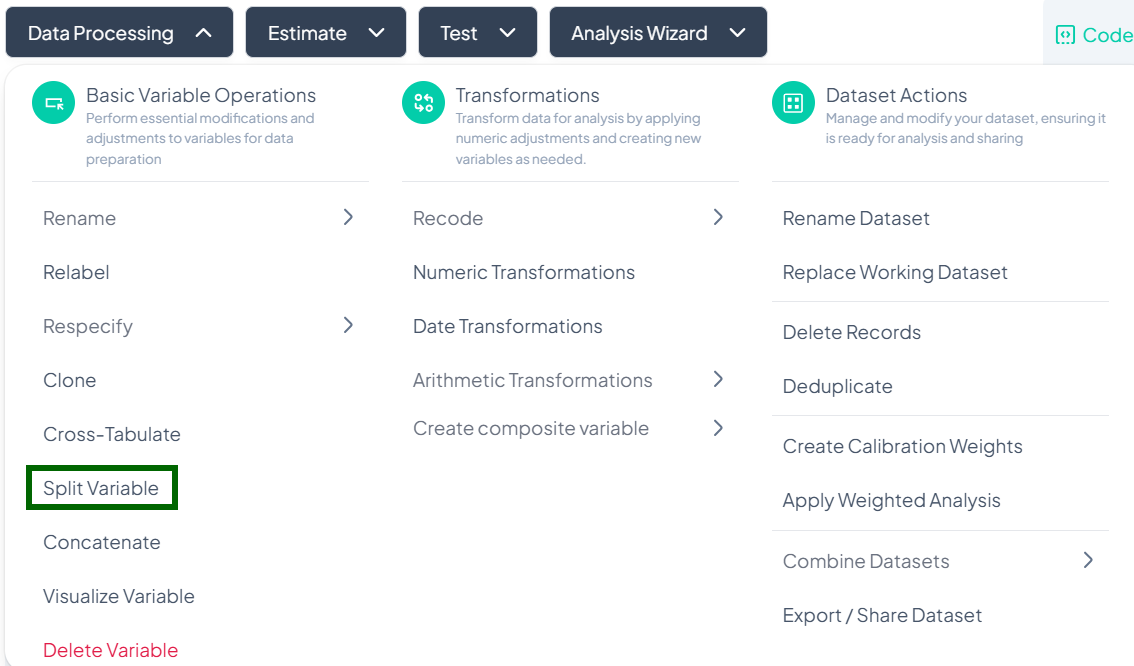
Split Variable

Within the Data Processing subsection of the Data Analysis module, the Split Variable tool allows you to break a single string or categorical variable into multiple new variables based on a specified delimiter. Follow the steps below to split one variable at a time.

Accessing the Split Variable Tool

1. Click Data Processing to expand the menu.
2. Under Basic Variable Operations, click Split Variable.

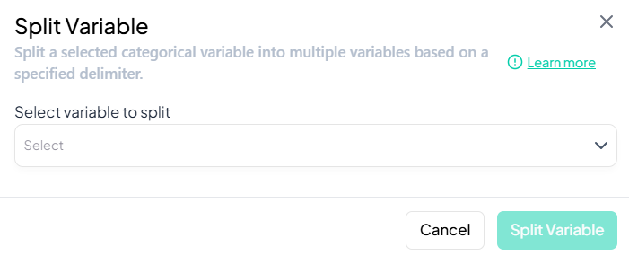
Splitting a Variable

Use this flow to divide one string or delimited categorical variable into multiple separate variables.

Step-by-Step Guide

1. Open Split Variable Modal

   • Data Processing → Basic Variable Operations → Split Variable

   

2. Select Variable

   • In the Select variable to split dropdown, choose the source variable (must be string or categorical with delimiters).

3. Specify Delimiter and Segments

   • After selecting the variable, additional fields appear:
     • Delimiter (e.g., comma, space, semicolon, or custom regex)
     • Number of segments or option to auto-detect the number of parts

4. Name New Variables

   • Provide base names for the output variables (e.g., 'address_part1', 'address_part2', …).

5. Confirm

   • Click Split Variable.
   • New columns are added to your dataset, each containing one segment of the original values.

   

Validation Rules

• Variable Type: Only variables of type String or Categorical with consistent delimiters can be split.
• Non-Empty Segments: If a row has fewer segments than specified, blank or missing values appear in the corresponding new columns.
• Unique Names: Each generated variable name must be unique within the dataset.

Tip:
Use Visualize Variable or a quick summary after splitting to verify that segments have been correctly parsed across your dataset.

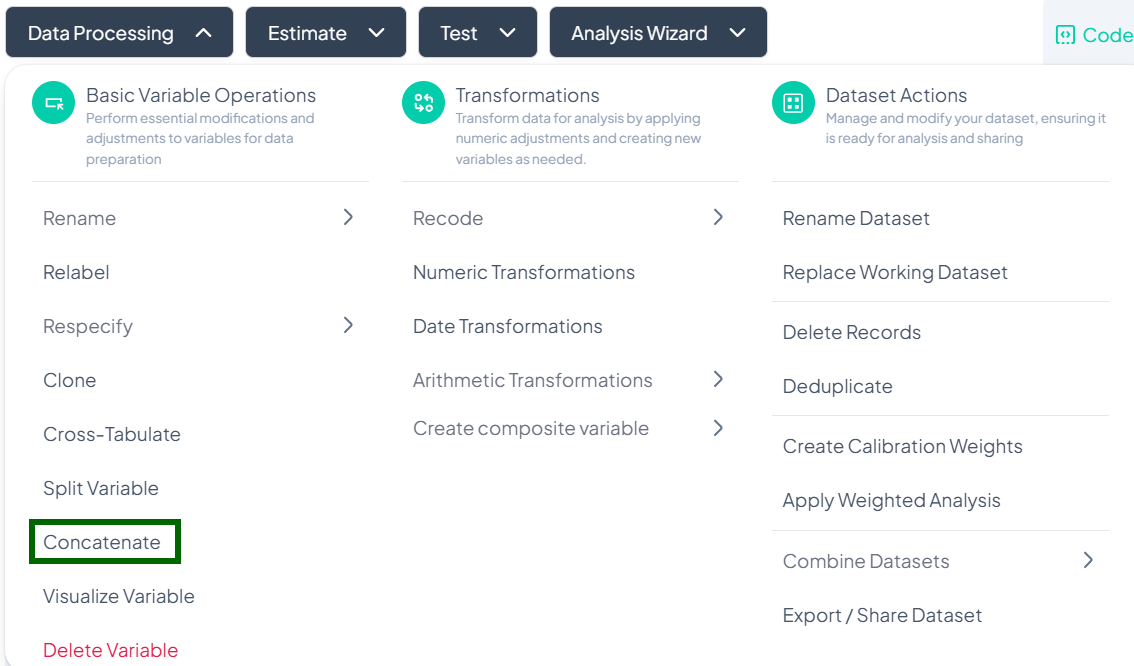
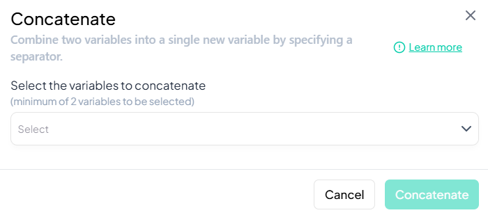
Concatenate

Within the Data Processing subsection of the Data Analysis module, the Concatenate tool lets you merge two or more existing variables into a single new variable, using a specified separator. Follow the steps below to concatenate multiple variables at once.

Accessing the Concatenate Tool

1. Click Data Processing to expand the menu.
2. Under Basic Variable Operations, click Concatenate.

Concatenating Variables

Use this flow to combine two or more string variables (or categorical variables treated as text) into a single new variable.

Step-by-Step Guide

1. Open Concatenate Modal

   • Data Processing → Basic Variable Operations → Concatenate

   

2. Select Variables

   • In the Select the variables to concatenate dropdown, choose two or more variables (e.g., 'first_name', 'last_name').

3. Specify Separator

   • After selecting variables, a Separator field appears. Enter the character(s) you want between values (e.g., space, comma, hyphen).

4. Name New Variable

   • In the New variable name field, type a unique name for the concatenated output (e.g., 'full_name').

5. Confirm

   • Click Concatenate.
   • A new column is added, containing the joined text for each row.

   

Validation Rules

• Variable Types: Only string or categorical variables may be concatenated.
• At Least Two: Must select a minimum of two variables.
• Unique Name: The new variable name must not duplicate existing names.

Tip:
After concatenation, use Visualize Variable or a quick frequency table to verify that the joined values appear as expected.

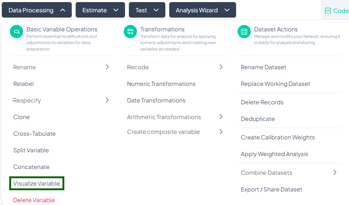
Visualize Variable

Within the Data Processing subsection of the Data Analysis module, the Visualize Variable tool lets you generate quick, customizable charts for any variable. Follow the steps below to create and adjust visualizations.

Accessing the Visualize Tool

1. Click Data Processing to expand the menu.
2. Under Basic Variable Operations, click Visualize Variable.

Creating a Visualization

Use this flow to produce a chart for any numeric or categorical variable.

Step-by-Step Guide

1. Open Visualization Modal

   • Data Processing → Basic Variable Operations → Visualize Variable

   

2. Select Variable

   • In the Select variable dropdown, choose the variable you wish to visualize (e.g., 'age').

3. Choose Chart Type

   • In the Select visualization type dropdown, pick one of the available options:
     • Bar Chart (default for categorical)
     • Column Chart
     • Pie Chart
     • Error Column
     • Box Plot (for continuous)

4. Render Chart

   • The chart auto-generates below the selectors.

Chart Types & Options

• Bar Chart
  Displays category counts or proportions.

• Column Chart
  Similar to bar chart, but vertical orientation.

• Pie Chart
  Shows category percentages.

• Error Column
  Displays means with error bars (e.g., CI or SD).

• Box Plot
  Summarizes continuous data distribution (median, quartiles, outliers).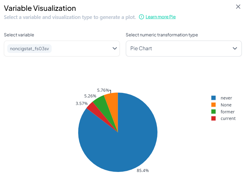

  

Post-Visualization Actions

• Adjust Bins / Categories: For histograms or box plots, change the number of bins or numeric range.
• Download Chart: Click the download icon on the chart to save as PNG or SVG.
• Customize Labels: Edit axis titles and legend labels directly in the modal.
• Push to Manuscript: Use the ••• menu to insert the chart into your manuscript draft.

Tip:
Combine Visualize Variable with Estimate outputs for powerful exploratory and descriptive workflows.

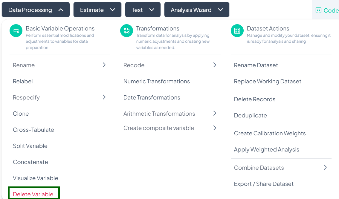
Delete Variable

Within the Data Processing subsection of the Data Analysis module, you can permanently remove unwanted variables from your working dataset. Follow the steps below to delete variables safely.

Accessing the Delete Tool

1. In the top-nav bar, click Data Processing to expand the menu.
2. Under Basic Variable Operations, scroll to the bottom and click Delete Variable.

Deleting Variables

Use this flow to remove one or more variables from your working dataset.

Step-by-Step Guide

1. Open Delete Modal

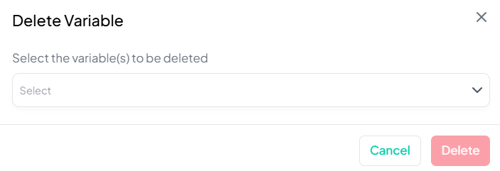
   • Data Processing → Basic Variable Operations → Delete Variable

   

2. Select Variable(s)

   • In the Select the variable(s) to be deleted dropdown, choose one or multiple variables.

3. Confirm Deletion

   • Click the red Delete button to remove the selected variable(s).

   

Warning & Recovery

⚠️ Warning: Deleting a variable removes it from the current working dataset. This action is irreversible in the session—deleted variables cannot be restored via the UI.

Recovery Options:

• If you deleted a variable by mistake, you must re-upload the original dataset or restore from a previously saved copy.
• Review your Analysis History to identify when the variable was removed and revert to an earlier dataset state if available.

2. Transformations

Transformations let you derive new variables or modify existing ones via numeric, date, arithmetic, and recoding operations.

Who Can Use Transformation Tools?

All project collaborators have access to transformation tools, but only those with edit permissions can apply irreversible changes like deletion.

Why It Matters

Transforming your data prepares it for meaningful analysis. These tools are designed for:

• Flexibility (visual or logic-based options)
• Transparency (actions tracked in history)
• Speed (no-code interface with point-and-click)

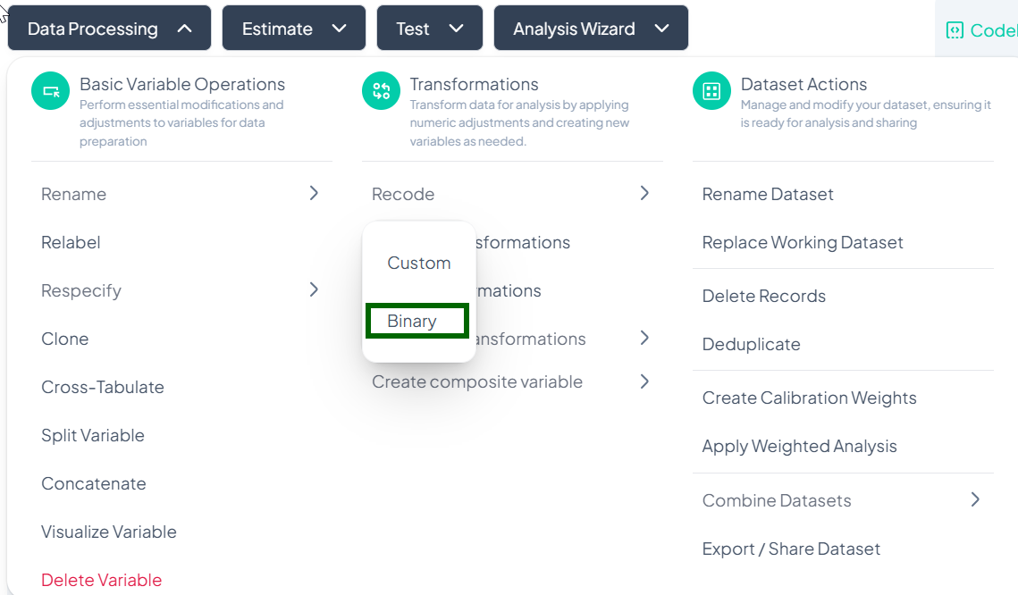
Recode

Within Data Processing → Basic Variable Operations, the Recode feature lets you collapse or remap values into new categories. You can choose a Custom recode for arbitrary groupings or a streamlined Binary recode for yes/no or presence/absence scenarios.

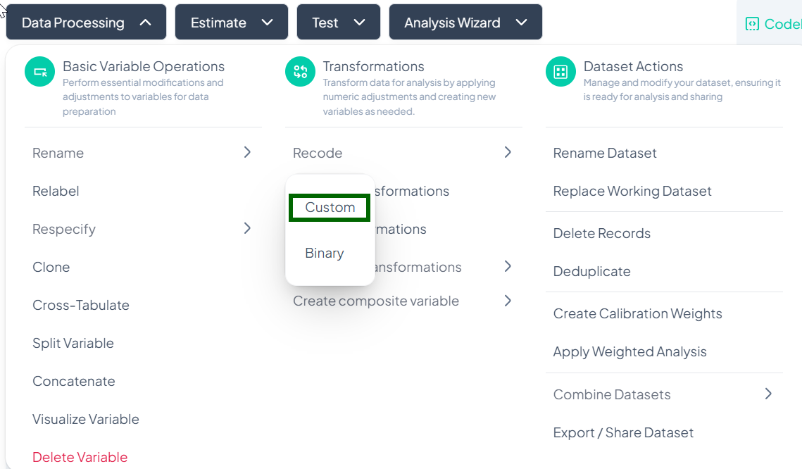
Accessing the Recode Tool

1. Click Data Processing → Basic Variable Operations.
2. Hover over Recode.
3. From the pop-out, choose Custom or Binary.

Custom Recode

Purpose

Use Custom when you need to map multiple original values into any number of new categories—for example, grouping age into decades or collapsing income brackets.

Step-by-Step Guide

1. Open Custom Recode

   • Data Processing → Basic Variable Operations → Recode → Custom

   

2. Switch Methods (optional)

   • Default is Visual Method (table-based).
   • Use the dropdown to switch to Syntax Method if you prefer writing rules.

3. Select Variable to Recode

   • Click the “Select variable to recode” dropdown and choose your source variable.

4. Enter Name for New Variable

   • In the “Enter name for the new variable” field, type a valid name.

5. Define Recoding Logic

   • In Visual Method: a table appears listing each original category—enter desired target category next to each value.
   • In Syntax Method: write your recode rules (e.g. 1,2 -> 'Low'; 3,4 -> 'High').

6. Proceed

   • Once mapping is complete, the Proceed button becomes active—click to generate the new recoded variable.

   

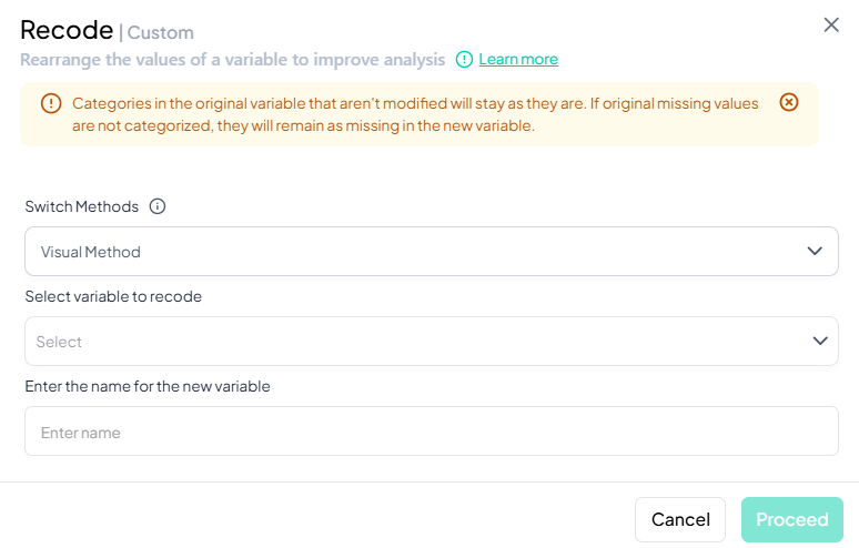
Notes & Validation

• Unmapped values remain as missing in the new variable.
• Original variable is unchanged; recode creates a brand-new column.
• Name validation: must be unique, ≤ 20 chars, letters/numbers/underscore only.

Binary Recode

Purpose

Use Binary to simplify a variable into two categories (e.g., “Yes” vs. “No,” “Present” vs. “Absent”). The UI guides you to pick which original values map to each binary outcome.

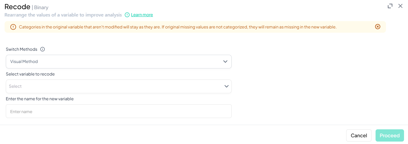
Step-by-Step Guide

1. Open Binary Recode

   • Data Processing → Basic Variable Operations → Recode → Binary

   

2. Switch Methods (optional)

   • Default Visual Method lists all unique values.
   • Syntax Method available for rule-based recoding.

3. Select Variable to Recode

   • From the dropdown, choose the source variable.

4. Enter Name for New Variable

   • Provide a valid target variable name.

5. Define Two Categories

   • In Visual Method: mark each original value as either Category 1 or Category 2.
   • In Syntax: write rules like '1,2 -> 0; 3,4 -> 1'.

6. Proceed

   • Click Proceed once both binary categories are fully specified.

   

Notes & Validation

• All values must be assigned to one of the two categories or treated as missing.
• New variable is boolean-style—ideal for prevalence or logistic analyses.
• Name rules: same as Custom Recode (unique, ≤ 20 chars, letters/numbers/underscore).

Tip: After recoding, use Visualize Variable to confirm the distribution of your new categories before proceeding with analysis.

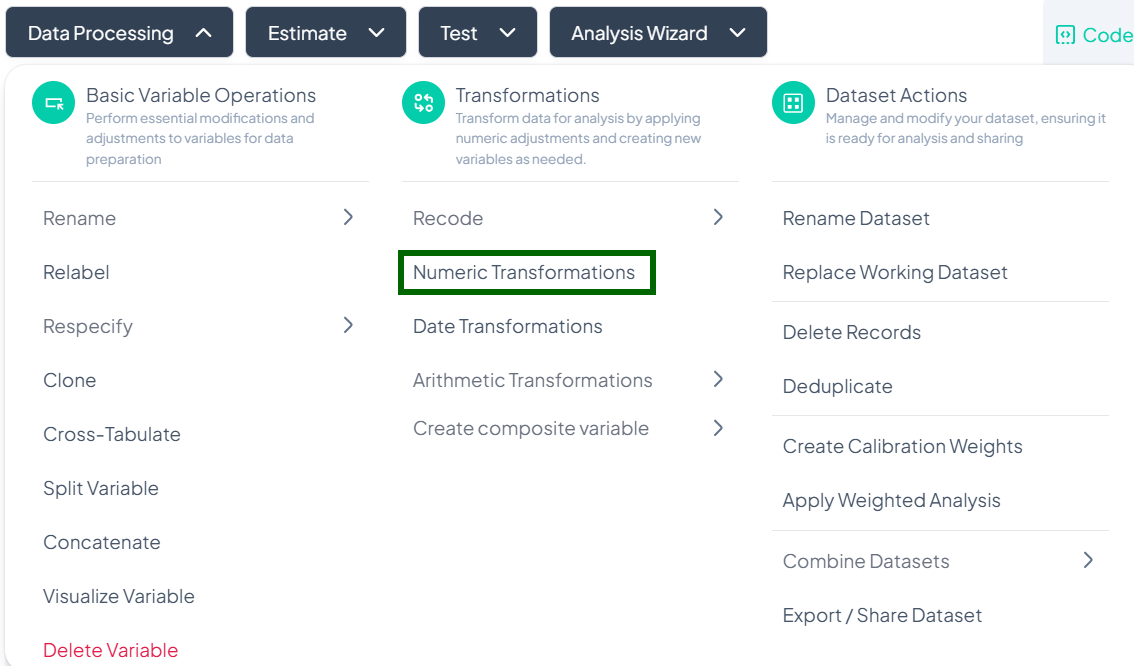
Numeric Transformations

Within the Data Processing subsection of the Data Analysis module, you can apply common numeric functions (log, square root, reciprocal, etc.) to one or more variables. Follow the steps below to derive new numeric variables without writing code.

Accessing Numeric Transformations

1. Click Data Processing to expand the menu.
2. Under Transformations, click Numeric Transformations.
3. The Numeric Transformation modal will open.

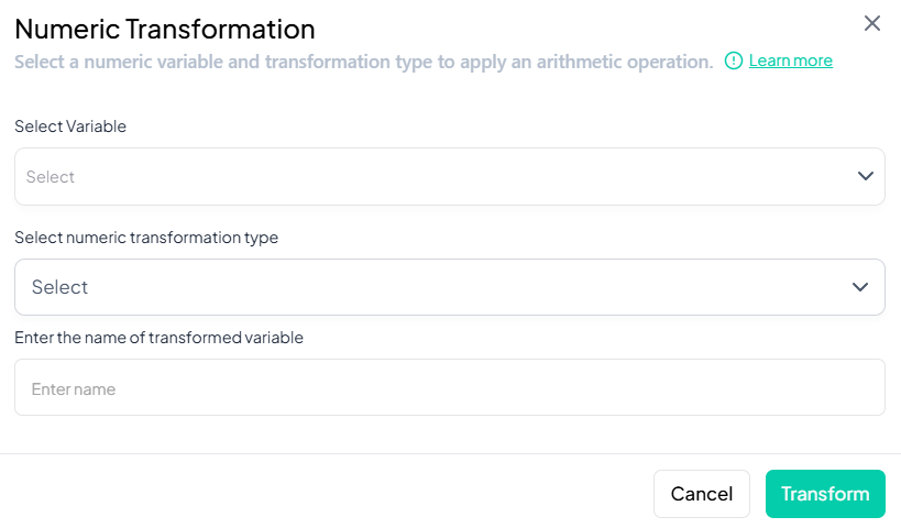
Single-Variable Numeric Transformation

Use this flow to apply a mathematical function to one variable and store the result in a new variable.

Step-by-Step Guide

1. Open Numeric Transformation

   • Data Processing → Transformations → Numeric Transformations

   

2. Select Variable

   • In the modal, click Select Variable and choose the numeric variable to transform.

3. Choose Transformation Type

   • Click Select numeric transformation type dropdown.
   • Options include:
     • Logarithm (natural log)
     • Square root
     • Square
     • Reciprocal (1/x)
     • Exponent
     • Cube
     • Z-score standardization

4. Name the Transformed Variable

   • In Enter name of transformed variable, type a unique name (e.g., 'log_income').

5. Execute Transformation

   • Click Transform.
   • A new variable with transformed values appears in your working dataset.

   

Validation Rules

• Variable Type: Source variable must be numeric (continuous or count).
• Unique Name: Transformed variable name must not duplicate any existing variable.
• Allowed Characters: A–Z, a–z, 0–9, and underscore ('_') only.
• Function Constraints:
  • Log and reciprocal require strictly positive input values.
  • Square root requires non-negative input values.

Tip:
After transforming, preview the new variable’s distribution (via Visualize Variable) to confirm that the operation produced the expected shape and range.

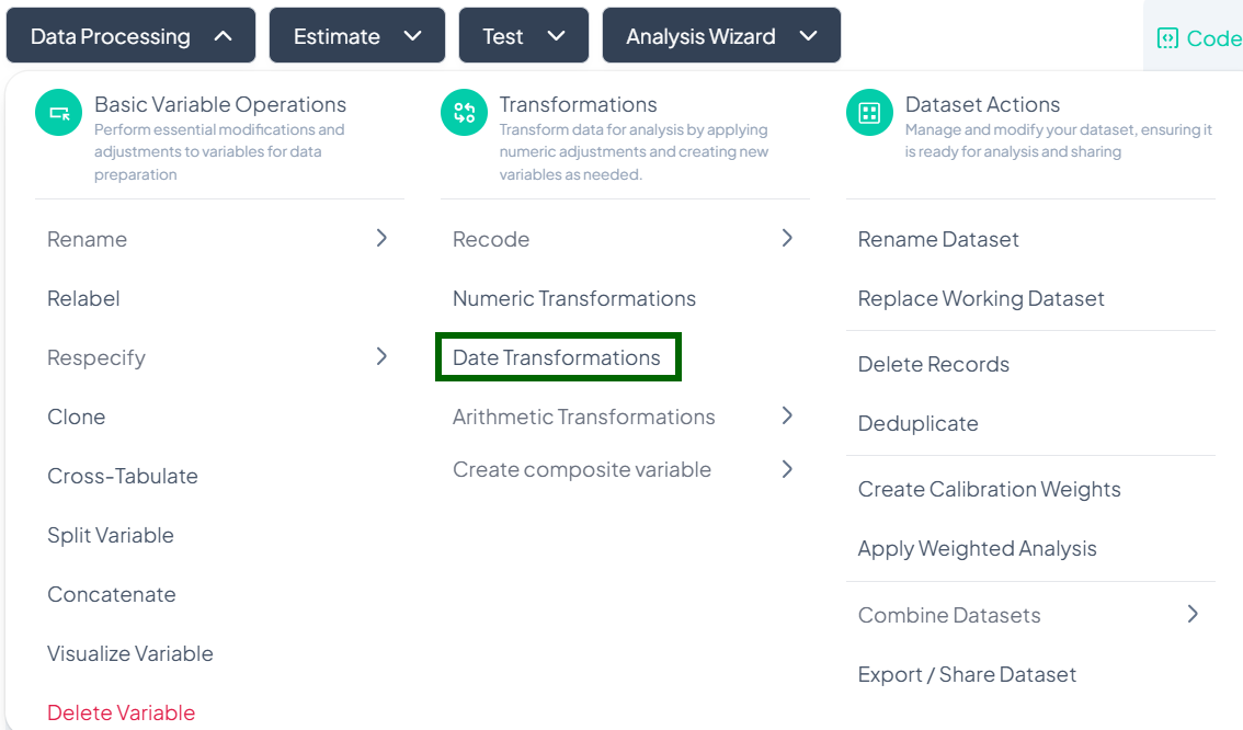
Date Transformations

Within the Data Processing subsection of the Data Analysis module, you can break down date variables into components or calculate intervals between dates. Follow the steps below to extract years, months, days, or compute elapsed time—all without writing code.

Accessing Date Transformations

1. Click Data Processing to expand the menu.
2. Under Transformations, click Date Transformations.
3. The Date Transformation modal will open.

Date Extraction

Use this flow to pull components (year, month, day) from a single date variable.

Step-by-Step Guide

1. Open Modal

   • Data Processing → Transformations → Date Transformations

   

2. Select Transformation Type

   • In Select date transformation type, choose Date Extraction.

3. Select Variable

   • Click Select Variable and pick the date variable to break down.

4. Choose Components

   • Tick one or more of:
     • Year
     • Month
     • Day

5. (Optional) Preview

   • Click Show Sample to view example output rows.

6. Extract

   • Click Extract.
   • New variable(s) appear for each selected component (e.g., 'var_year', 'var_month').

   

Validation Rules

• Variable Type: Source must be a valid date or datetime.
• Component Selection: At least one of Year, Month, or Day must be checked.
• Output Naming: System auto-appends '_year', '_month', '_day' to the original name.

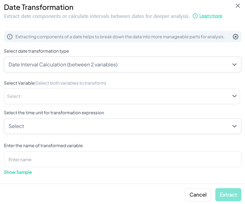
Interval Between Two Date Variables

Use this flow to compute the time difference between two date variables.

Step-by-Step Guide

1. Open Modal

   • Data Processing → Transformations → Date Transformations

2. Select Transformation Type

   • Choose Date Interval Calculation (between 2 variables).

3. Select Variables

   • Click Select Variable and choose both date variables (order matters: later date minus earlier date).

4. Select Time Unit

   • In Select the time unit for transformation expression, choose one of:
     • Days
     • Months
     • Years

5. Name Transformed Variable

   • Enter a unique name (e.g., 'interval_days').

6. (Optional) Preview

   • Click Show Sample to verify sample calculations.

7. Extract

   • Click Extract.
   • A new interval variable appears with elapsed time in the chosen unit.

   

Validation Rules

• Both Variables: Must be date or datetime types.
• Order: The first selected variable should represent the earlier date.
• Unit Choice: Only one time unit may be selected.
• Name Uniqueness: New variable name must not duplicate existing names.

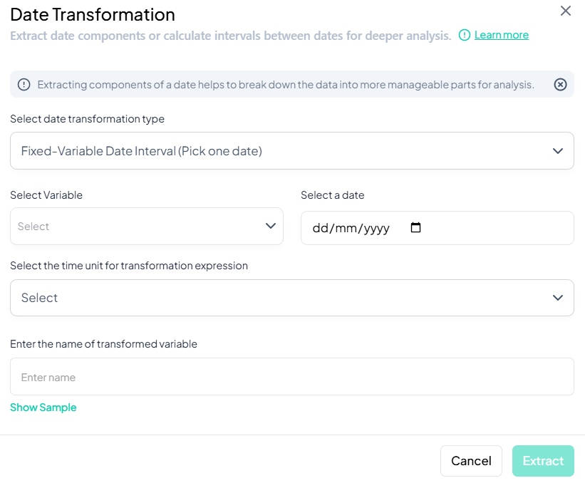
Fixed-Date Interval Calculation

Use this flow to calculate the elapsed time between each observation’s date and a single fixed reference date.

Step-by-Step Guide

1. Open Modal

   • Data Processing → Transformations → Date Transformations

2. Select Transformation Type

   • Choose Fixed-Variable Date Interval (Pick one date).

3. Select Variable & Reference Date

   • Select Variable: pick the date variable to compare.
   • Select a date: click the calendar icon to choose the reference date (e.g., project start date).

4. Select Time Unit

   • Choose Days, Months, or Years for the interval.

5. Name Transformed Variable

   • Enter a clear name (e.g., 'days_since_start').

6. (Optional) Preview

   • Click Show Sample to inspect a few rows of output.

7. Extract

   • Click Extract.
   • A new variable is added with interval values relative to the fixed date.

   

Validation Rules

• Variable Type: Source must be date or datetime.
• Reference Date: Must be a valid calendar date.
• Unit Selection: Only one time unit allowed.
• Naming: New variable name must be unique and follow naming conventions.

Tip:
Use date transformations to standardize time-based analyses—then visualize trends over time with the Estimate module’s trend analysis or line charts.

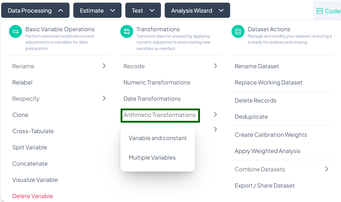
Arithmetic Transformations

Within the Data Processing subsection of the Data Analysis module, you can apply arithmetic operations—either against a constant or between two or more variables—to generate new computed fields. Follow the steps below to scale, combine, or adjust values without writing any code.

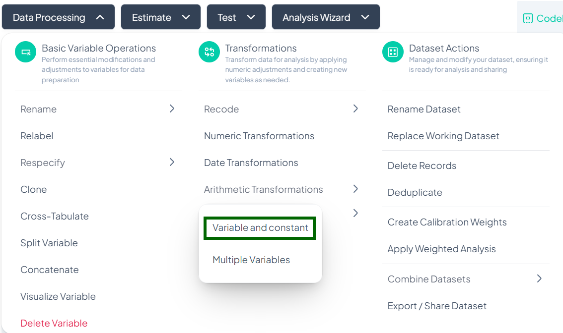
Accessing Arithmetic Transformations

1. Click Data Processing to expand the menu.
2. Under Transformations, click Arithmetic Transformations.
3. Choose Variable and constant or Multiple Variables from the pop-out.

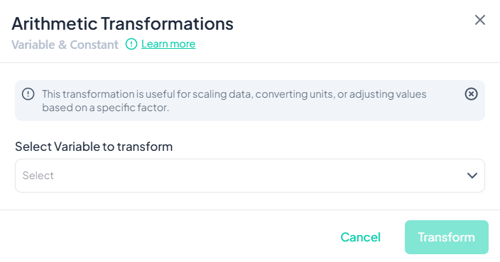
Variable & Constant Transformation

Use this flow to apply an arithmetic operation between a single variable and a constant (e.g., convert units, offset values).

Step-by-Step Guide

1. Open Modal

   • Data Processing → Transformations → Arithmetic Transformations → Variable and constant

   

2. Select Variable

   • In the Select Variable to transform dropdown, choose the source variable.

3. Choose Operation & Enter Constant

   • An operation selector appears next to the variable name. Click it and pick one of:
     • + Sum
     • − Subtract
     • × Multiply
     • ÷ Divide
   • In the adjacent field, type the constant value (e.g., '1000' to convert from grams to kilograms).

4. Name Transformed Variable

   • Scroll down (if needed) and enter a unique name for the new variable (e.g., 'weight_kg').

5. Execute Transformation

   • Click Transform.
   • A new variable appears in your dataset with the computed values.

   

Validation Rules

• Source Type: Variable must be numeric.
• Constant: Must be a valid number.
• Unique Name: Transformed variable name must not duplicate existing variables.
• Operation Constraints:
  • Division by zero is not allowed.
  • Large constants may affect numeric precision.

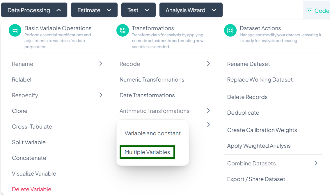
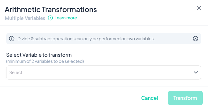
Multiple-Variable Transformation

Use this flow to combine two or more numeric variables using arithmetic operations (e.g., add survey subscales, compute total score).

Step-by-Step Guide

1. Open Modal

   • Data Processing → Transformations → Arithmetic Transformations → Multiple Variables

   

2. Select Variables

   • Click Select Variable to transform and choose at least two numeric variables.

3. Choose Operation

   • In Enter Operator, pick one of:
     • + Sum
     • − Subtract
     • × Multiply
     • ÷ Divide
   • Note: Divide and subtract operations must be between exactly two variables; sum and multiply can include more.

4. Review Expression

   • A preview of the expression appears below—confirm the order and operation.

5. Name Transformed Variable

   • Enter a unique name (e.g., 'total_score') in the name field.

6. Execute Transformation

   • Click Transform.
   • The new combined variable is added to your dataset.

   

Validation Rules

• Variable Count:
  • Sum/Multiply: at least two variables.
  • Subtract/Divide: exactly two variables.
• Source Type: All selected variables must be numeric.
• Unique Name: Cannot match existing variable names.
• Operator Constraints:
  • Division by zero prohibited.
  • Order of operations follows left-to-right selection.

Tip:
Preview a few rows of the expression by toggling the Preview mock data switch (if available) before committing the transformation.

Create Composite Variables

Within the Data Processing subsection of the Data Analysis module, you can build new composite variables either by combining categories under conditional logic or by generating all unique category combinations. Follow the steps below to leverage both methods without writing any code.

Accessing Create Composite Variable

1. Click Data Processing to expand the menu.
2. Under Transformations, click Create composite variable.
3. Select either Using conditions or Unique Combinations from the pop-out.

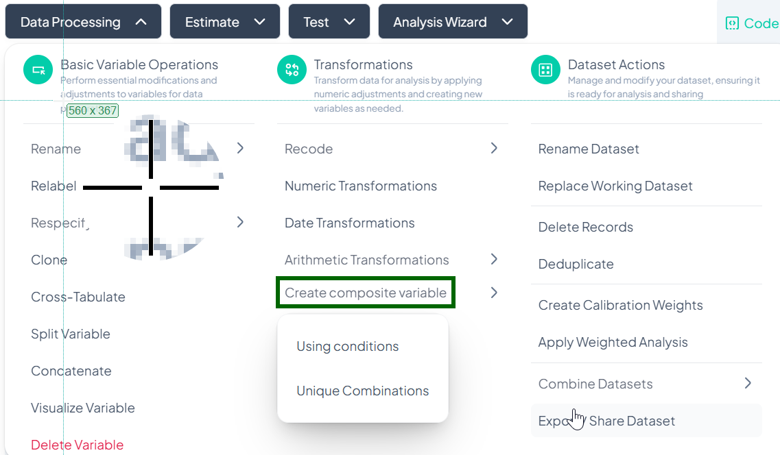
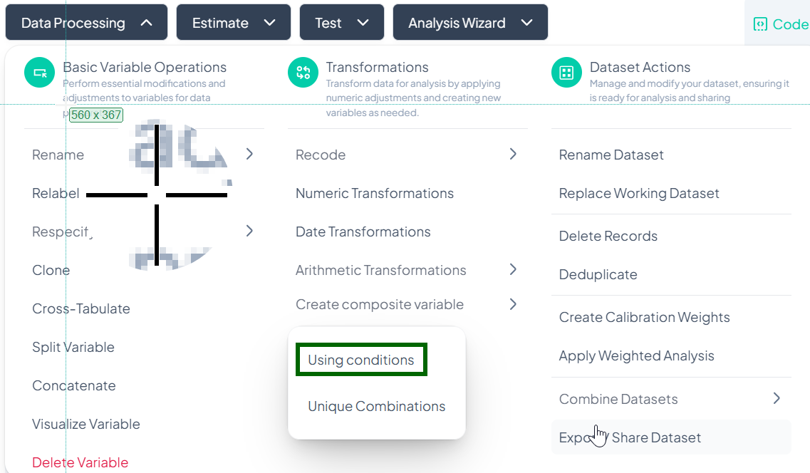
Using Conditions

Use this method to merge or recode values based on conditional logic (e.g., “Male AND Smoker” → “Male Smoker”).

Step-by-Step Guide

1. Open Modal

   • Data Processing → Transformations → Create composite variable → Using conditions

   

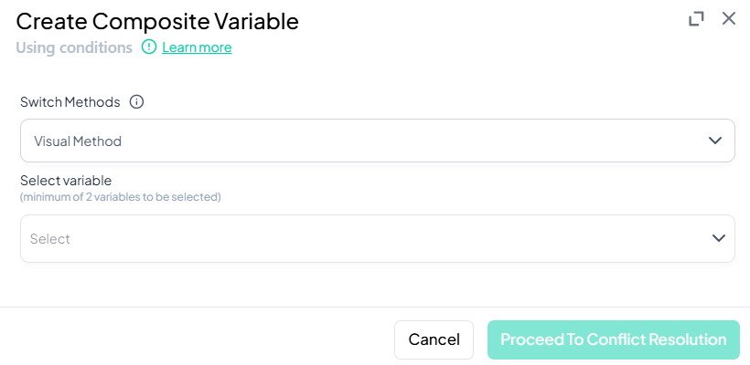
2. Switch Method (Optional)

   • In Switch Methods, pick Visual Method or Classic Method.
     • Visual: drag-and-drop groups.
     • Classic: write logical expressions.

3. Select Variables

   • Click Select variable and choose two or more source variables.

4. Define Composite Logic

   • Visual Method:
     • Drag category “blocks” into a merged group area.
     • Label the new composite category.
   • Classic Method:
     • Enter conditions using logical operators (e.g., 'sex == 1 AND smoker == 1').
     • Assign a label for each rule.

5. Resolve Conflicts

   • Click Proceed To Conflict Resolution.
   • If any observation matches multiple rules, decide precedence or default category.

6. Save Composite Variable

   • After conflict resolution, confirm to create the new variable.

Validation Rules

• Minimum Variables: At least two source variables required.
• Coverage: Every possible combination should be assigned or explicitly marked missing.
• Unique Labels: Composite category labels must be distinct.
• Logical Consistency: Classic expressions must reference valid variable names and values.

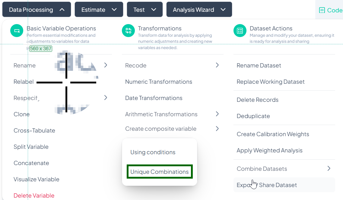
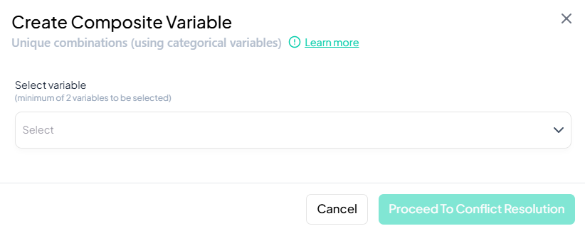
Unique Combinations

Use this method to automatically generate a new variable representing every unique combination of selected categorical variables (e.g., 'Region' + 'Gender' → 'Region_Gender').

Step-by-Step Guide

1. Open Modal

   • Data Processing → Transformations → Create composite variable → Unique Combinations

   

2. Select Variables

   • In Select variable, choose two or more categorical variables.

3. Name Transformed Variable

   • (Optional) If prompted, enter a name for the new composite variable (e.g., 'region_gender').

4. Proceed to Conflict Resolution

   • Click Proceed To Conflict Resolution.
   • Review automatically generated combinations and adjust labels if desired.

5. Save Composite Variable

   • Confirm to add the new variable containing unique category combinations.

   

Validation Rules

• Variable Type: Only categorical variables may be selected.
• Minimum Variables: At least two variables required to form combinations.
• Name Uniqueness: New variable name must not conflict with existing names.
• Label Clarity: Composite labels are auto-generated by concatenating original values; edit if needed for readability.

Tip:
After creating a composite variable, use Visualize Variable or Cross-Tabulate to verify that all combinations appear as expected.

3. Dataset-Level Actions

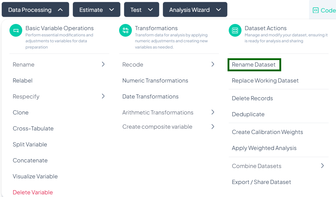
Rename Dataset

Within the Data Processing subsection of the Data Analysis module, you can update the dataset’s label to make it more descriptive and easy to identify. Follow the steps below to rename your working dataset.

Accessing the Rename Dataset Tool

1. Click Data Processing to expand the menu.
2. Scroll down to the Dataset Actions section.
3. Click Rename Dataset.

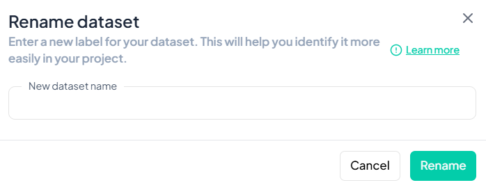
Step-by-Step Guide

1. Launch Rename Modal

   • Data Processing → Dataset Actions → Rename Dataset

   

2. Enter New Dataset Name

   • In the New dataset name field, type a descriptive title for your dataset.

3. Save Changes

   • Click the green Rename button.
   • The dataset label updates immediately across the project.

   

Validation Rules

• Unique: The new name must not duplicate any existing dataset label in your project.
• Allowed Characters: Letters, numbers, spaces, hyphens ('-'), and underscores ('_').
• Length: Maximum of 50 characters.

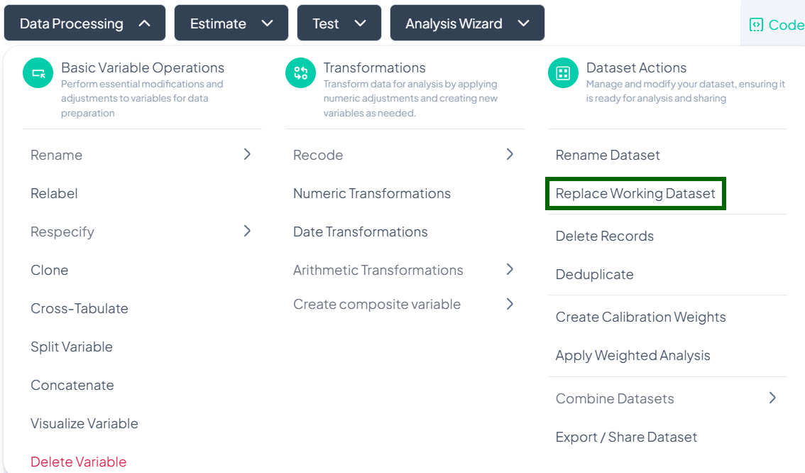
Replace Working Dataset

When you need to swap out your current dataset for a new file or an existing project file, use the Replace Working Dataset action. This ensures your analyses run on the correct data without creating a new project.

Accessing the Replace Dataset Tool

1. Click Data Processing to expand the menu.
2. Scroll to Dataset Actions.
3. Click Replace Working Dataset.

Step-by-Step Guide

1. Launch the Replace Dataset modal

   • Data Processing → Dataset Actions → Replace Working Dataset

   

2. Select Source

   • In the Upload File dialog, switch between tabs:
     • Recent Files
     • My Storage
     • Upload (to browse your local device)

3. Choose Your File

   • Check the box next to the desired file (CSV, XLSX, etc.).

4. Confirm Replacement

   • Click Import (or Upload) at the bottom.
   • The new dataset replaces the working dataset; existing transformations remain intact but will apply to the new data.

   

Important Notes

• One file at a time: You can only replace with a single file in each operation.
• Data schema changes: If the new dataset has different variable names or types, you may need to re-run or adjust prior processing steps (e.g., recodes, labels).
• History tracking: The replacement is logged in the Analysis History; you can review when the dataset swap occurred.
• Permissions: Only users with Project Owner or Edit privileges can replace the working dataset.

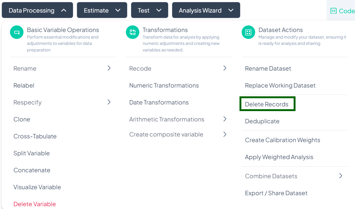
Delete Records

Use the Delete Records action to remove unwanted rows based on specified conditions. This is useful for excluding outliers, incomplete entries, or participants outside your study criteria.

Accessing the Delete Records Tool

1. Click Data Processing to expand the menu.
2. Scroll down to Dataset Actions.
3. Click Delete Records.

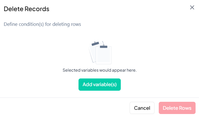
Step-by-Step Guide

1. Launch the Delete Records modal

   • Data Processing → Dataset Actions → Delete Records

   

2. Add Condition Variables

   • Click Add variable(s).
   • In the picker, select one or more variables you will use to define deletion criteria (e.g., 'age', 'income').

3. Define Delete Conditions

   • For each chosen variable, set a logical condition (e.g., 'age < 18', 'income = 0').
   • Use AND / OR operators to combine multiple conditions.

4. Preview Matches (if available)

   • After defining conditions, a live count or preview of matching rows may appear.

5. Delete Rows

   • When ready, click the Delete Rows button.
   • Confirm the action in the prompt to permanently remove those records from the working dataset.

   

Important Notes & Warnings

• Irreversible in Session: Once rows are deleted, they cannot be recovered in the current session. Use Export or Clone beforehand if you might need the full dataset later.
• Validation: The Delete Rows button stays disabled until at least one valid condition is defined.
• Permissions: Only users with Edit or Project Owner rights can delete records.
• History Logged: Deletion actions are recorded in the Analysis History for audit and reproducibility.

Warning:
Deleting records can significantly impact your results. Always review and export a backup of your data before proceeding.

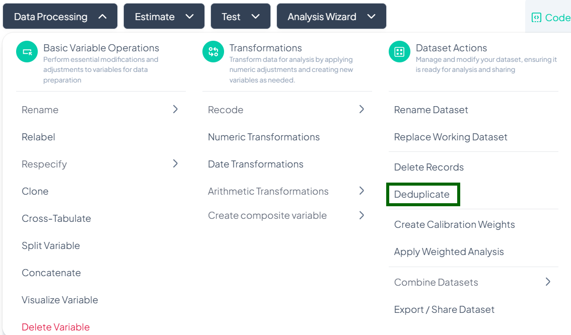
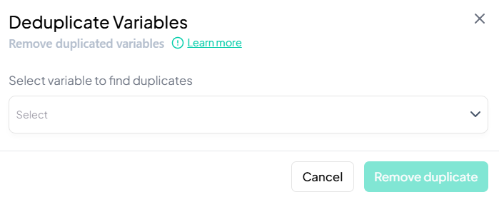
Deduplicate

Use the Deduplicate action to identify and remove duplicate columns from your working dataset. This helps maintain a clean variable set and prevents redundant analyses.

Accessing the Deduplicate Tool

1. Click Data Processing to expand the menu.
2. Scroll down to Dataset Actions.
3. Click Deduplicate.

Step-by-Step Guide

1. Launch the Deduplicate modal

   • Data Processing → Dataset Actions → Deduplicate

   

2. Select Variable to Scan

   • In the Deduplicate Variables modal, click the dropdown and choose the variable you suspect has duplicates (e.g., 'participant_id').

3. Review Duplicate Set

   • The system scans for repeated values in the selected column and displays all matching variable pairs.

4. Remove Duplicates

   • Click Remove duplicate to drop the redundant variables from your working dataset.

   

Important Notes & Warnings

• Non-Destructive: Removing duplicates only affects your working dataset. The original import remains intact.
• Confirmation Prompt: A confirmation is required before any variable is removed.
• Audit Trail: Deduplication actions are logged in the Analysis History for traceability.
• Permissions: Only users with Edit or Project Owner rights can deduplicate variables.

Tip:
After deduplicating, run a quick Visualize Variable or Cross-Tabulate on the remaining column to ensure data integrity.

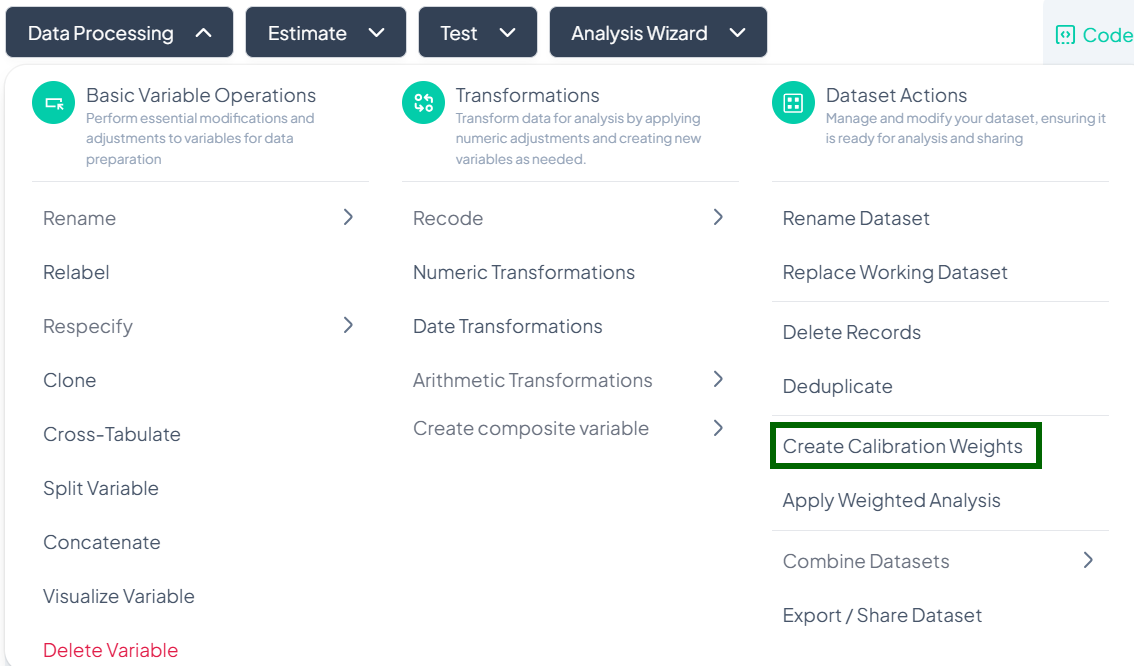
Create Calibration Weights

Use the Create Calibration Weights action to generate post-stratification or raking weights that align your sample with known population benchmarks. This ensures survey estimates more accurately reflect the target population.

Accessing the Calibration Weights Tool

1. Click Data Processing to expand the menu.
2. Scroll down to Dataset Actions.
3. Click Create Calibration Weights.

Step-by-Step Guide

1. Launch the Create Calibration Weights modal

   • Data Processing → Dataset Actions → Create Calibration Weights

   

2. Enter New Variable Label

   • In the New Variable Label field, type a descriptive name for your weight variable (e.g., 'pop_rake_weight').

3. Choose Base Variable

   • From the “Choose the variable to be used in creating the weights” dropdown, select the survey variable that corresponds to the benchmark distribution (e.g., 'age_group').

4. Add Weight Entries

   • Click + Add New Weight Entry to define each subgroup’s target proportion.
   • For each entry, select a category (e.g., '18–24', '25–34') and enter its target percentage (must sum to 100%).

5. Generate Weights

   • Once all entries are filled and validations pass, click Generate Weight.
   • Chisquares computes the calibration factors and adds a new weight variable to your dataset.

   

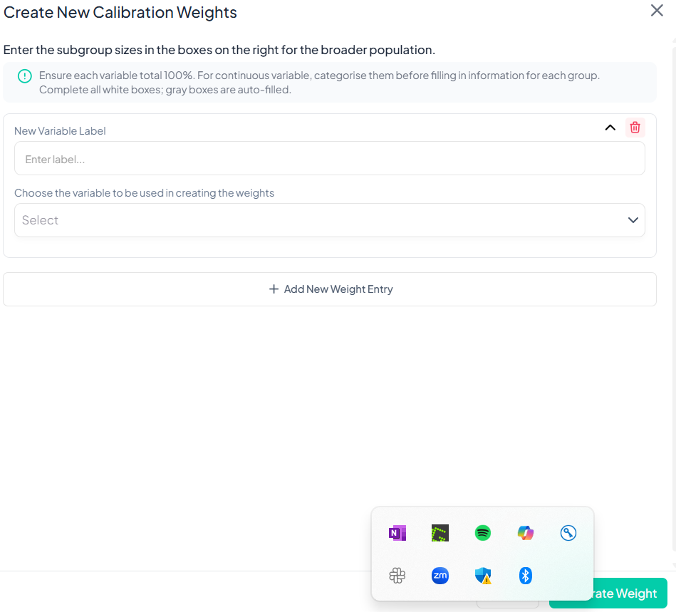
Key Considerations

• Sum to 100%: Ensure the target proportions across all subgroups total exactly 100%.
• Categorical Variables: If your benchmark variable is continuous, recode it into categories first.
• Auto-Filled Entries: Gray boxes represent automatically computed totals; only white boxes require input.
• Reproducibility: All weight creation steps are logged in the Analysis History.
• Permissions: Only users with Edit or Owner roles can generate weights.

Tip:
After creating weights, apply them via Dataset Actions → Apply Weighted Analysis before running your next Estimate or Test to incorporate the calibration in all analyses.

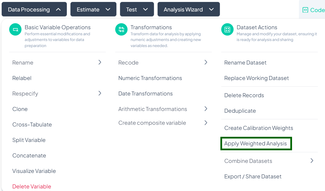
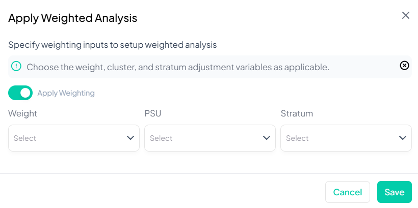
Apply Weighted Analysis

Use the Apply Weighted Analysis action to incorporate survey design weights (and optional clustering/stratification variables) into all subsequent estimates and tests.

Accessing the Weighted Analysis Tool

1. Click Data Processing to expand the menu.
2. Scroll down to Dataset Actions.
3. Click Apply Weighted Analysis.

Step-by-Step Guide

1. Open the Apply Weighted Analysis modal

   • Data Processing → Dataset Actions → Apply Weighted Analysis

   

2. Toggle Weighting On

   • Switch Apply Weighting to the On position (green).

3. Select Weight Variable

   • In the Weight dropdown, choose your calibration or sampling weight variable (e.g., 'pop_rake_weight').

4. (Optional) Specify PSU

   • If your survey uses clustering, select the Primary Sampling Unit variable under PSU.

5. (Optional) Specify Stratum

   • If stratified sampling was used, select the Stratum variable under Stratum.

6. Save Settings

   • Click Save to apply weights and design settings to your working dataset.

   

Key Notes & Best Practices

• Global Effect: Once saved, all Estimate and Test analyses use the specified weight and design by default.
• Preview Impact: Review your first weighted estimate to confirm expected changes (e.g., adjusted means or proportions).
• Cluster & Stratum Optional: If PSU or Stratum are left blank, only the weight will be applied.
• Permissions: Only users with Edit or Owner roles can modify weighted analysis settings.
• Reproducibility: All weight and design settings are recorded in Analysis History for auditing.

Tip:
To temporarily disable weighting for a specific analysis, toggle the Apply Weighting switch off, then re-enable afterward.

Combine Datasets

The Combine Datasets feature under Dataset Actions lets you join multiple files either by appending (stacking different individuals) or merging (joining on the same individuals).

Accessing Combine Datasets

1. Click Data Processing to expand the menu.
2. Scroll down to Dataset Actions.
3. Click Combine Datasets.

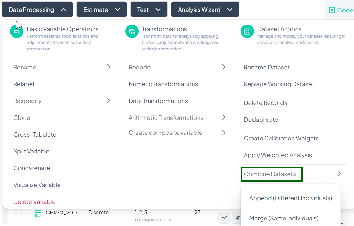
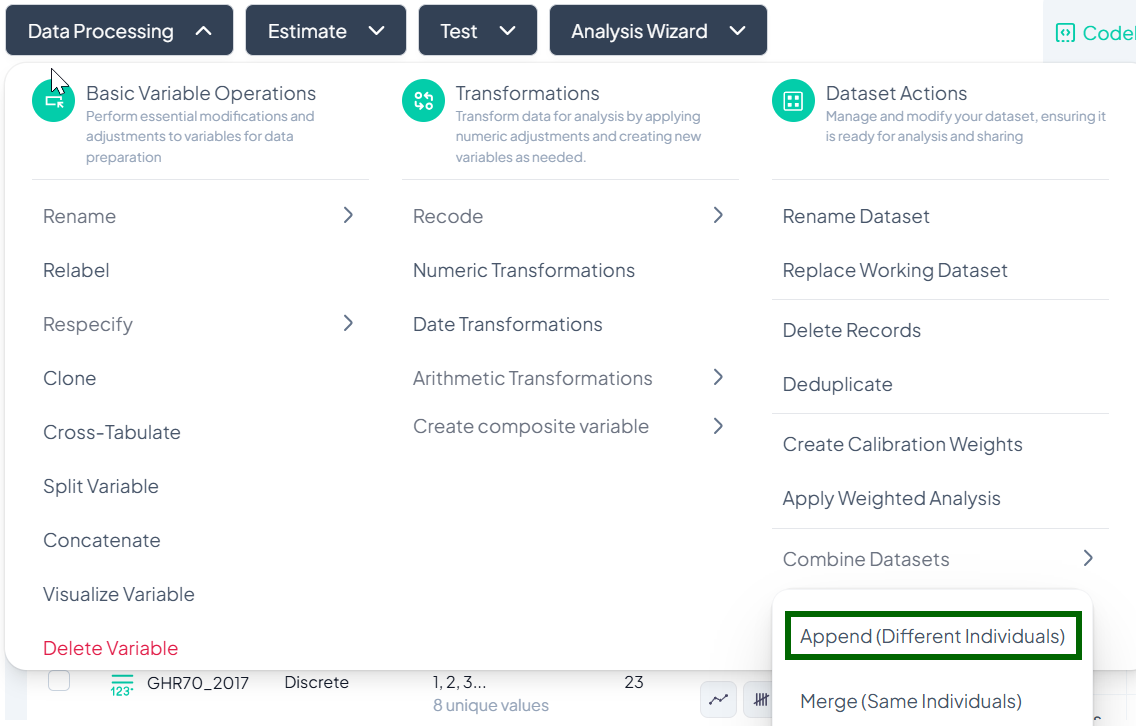
Append Datasets (Different Individuals)

Use Append when you have two (or more) datasets containing different records—e.g., additional survey respondents—and you want to stack them into one larger dataset.

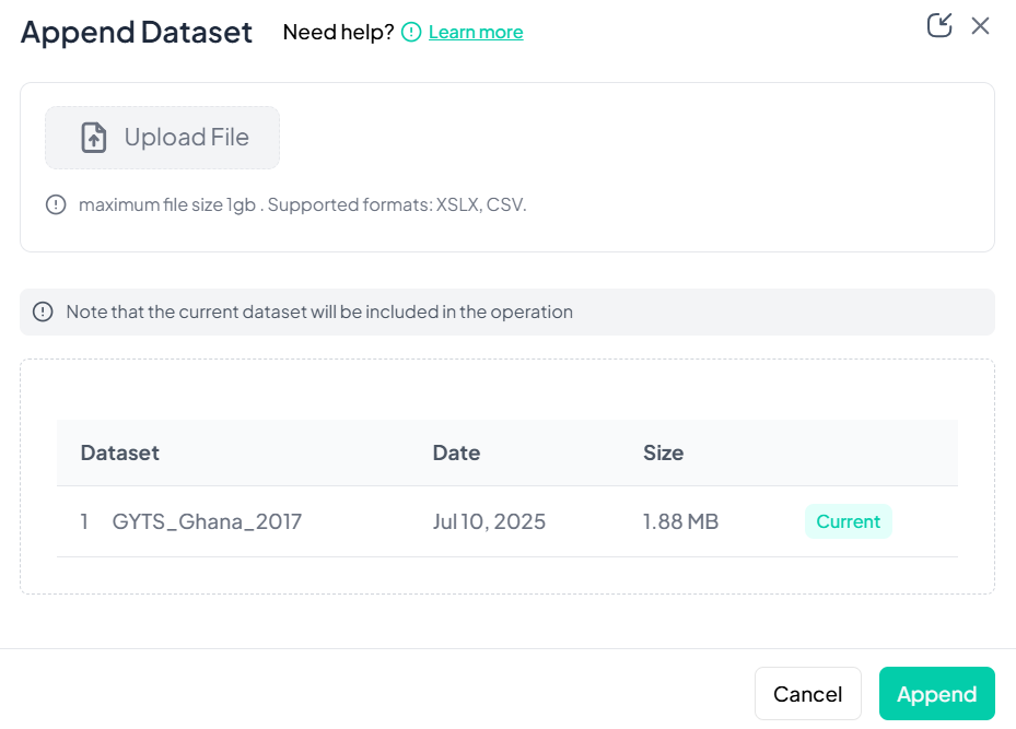
Step-by-Step Guide

1. Select Append

   • Data Processing → Dataset Actions → Combine Datasets → Append (Different Individuals)

   

2. Upload the Second File

   • In the Append Dataset modal, click Upload File and choose your CSV/XLSX.
   • Maximum size: 1 GB.

3. Confirm Included Datasets

   • The current project dataset appears in the list automatically.
   • Your newly uploaded file appears below once upload completes.

4. Execute Append

   • Click Append.
   • Chisquares concatenates the rows from both files into one working dataset.

   

Notes & Tips

• Column Alignment: Variables must have matching names and types to align correctly.
• Missing Columns: If one dataset lacks a column, the appended rows will show missing values (NA) in that column.
• Backup: Consider renaming your original dataset before appending for easy rollback.

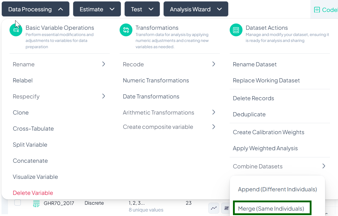
Merge Datasets (Same Individuals)

Use Merge when you have two datasets containing the same units of analysis—e.g., baseline and follow-up data—and you wish to join them on a key variable.

Step-by-Step Guide

1. Select Merge

   • Data Processing → Dataset Actions → Combine Datasets → Merge (Same Individuals)

   

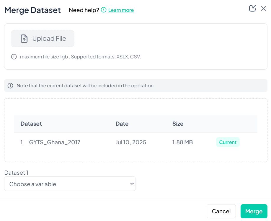
2. Upload the Second File

   • In the Merge Dataset modal, click Upload File and choose your CSV/XLSX.

3. Confirm Included Datasets

   • The current dataset is listed first; your uploaded file appears below.

4. Choose Merge Key

   • Under Dataset 1, select the key variable to match on (e.g., 'participant_id').
   • Under Dataset 2, select its corresponding key variable.

5. Execute Merge

   • Click Merge.
   • Chisquares performs a left join, adding new columns from Dataset 2 to Dataset 1 by matching key values.

   

Notes & Tips

• Join Types: Currently Chisquares uses a left-join; unmatched rows in Dataset 2 will produce missing values.
• Key Validation: Ensure the key variable is unique within each dataset to avoid unintended record duplication.
• Preview: Use the Show Sample link (if available) to confirm matching before final merge.

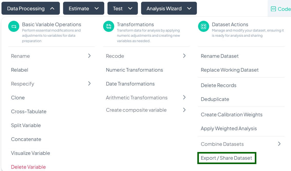
Export/Share Dataset

Use the Export / Share Dataset action to download your processed dataset or share it with collaborators via link, email, or third-party storage.

Accessing the Export / Share Tool

1. Click Data Processing to expand the menu.
2. Scroll to Dataset Actions.
3. Click Export / Share Dataset.

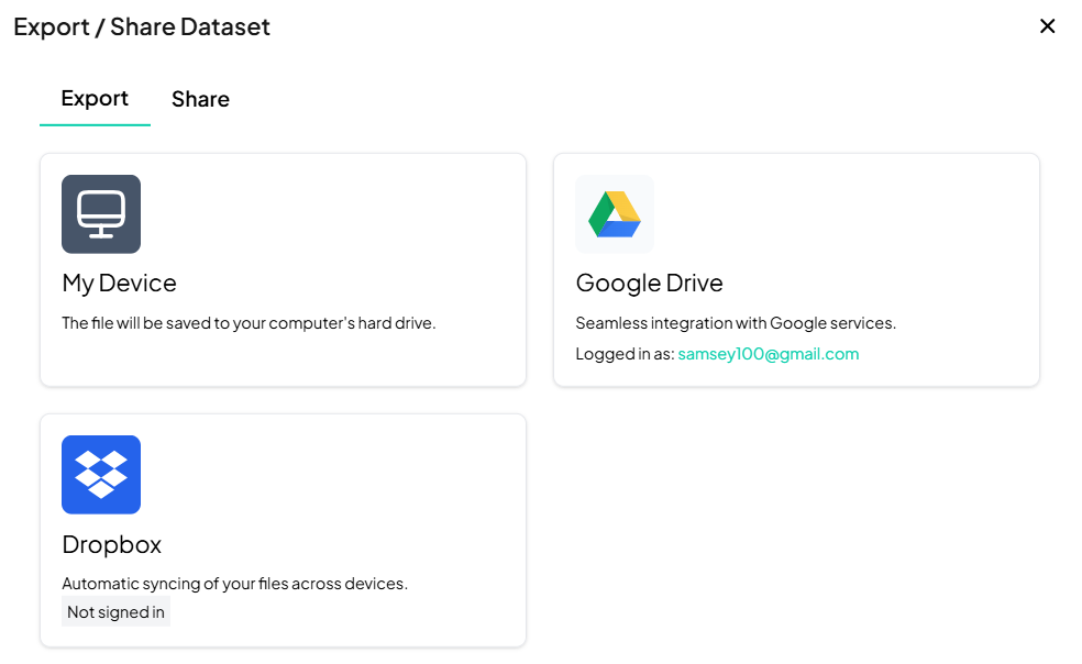
Exporting Your Dataset

Step-by-Step Guide

1. Open Export modal

   • Data Processing → Dataset Actions → Export / Share Dataset (Export tab opens by default).

2. Choose Export Destination

   • My Device: Download directly to your computer.
   • Google Drive: Save to your connected Google account.
   • Dropbox: Save to your Dropbox (sign in if prompted).

   

3. Initiate Export

   • Click the tile for your desired destination.
   • Follow any prompts (e.g., signin, folder selection).
   • Confirm to start the download or transfer.

Best Practices

• File Format: Chisquares exports in CSV by default—rename extension as needed for Excel.
• Storage Quota: Ensure your Google Drive/Dropbox has sufficient space.
• Download Verification: After exporting, open the file to verify row/column counts match expectations.

Sharing Your Dataset

Step-by-Step Guide

1. Switch to Share Tab

   • In the Export / Share Dataset modal, click Share.

2. Generate Shareable Link

   • In the Share the document as link field, choose link privacy (View only / Editor).
   • Click Copy Link to copy to clipboard.

   

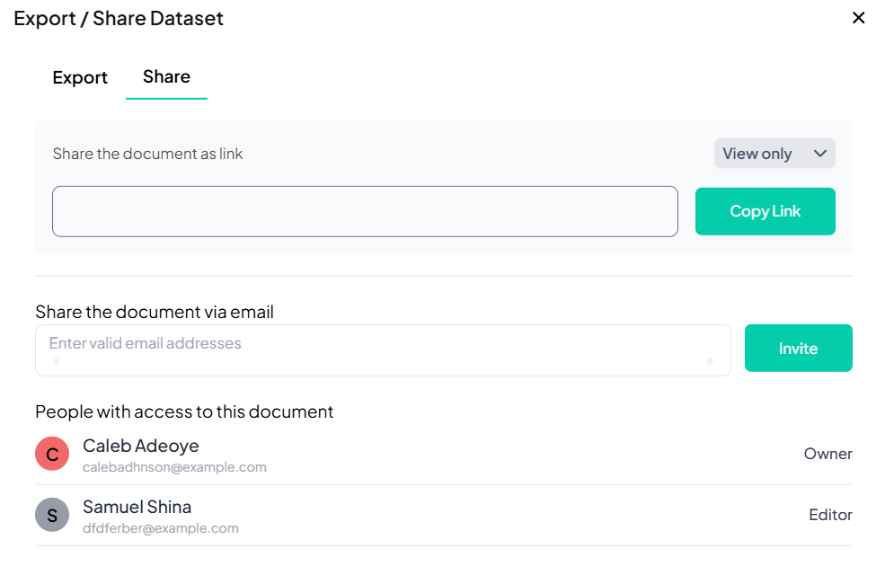
3. Invite via Email

   • Under Share the document via email, enter one or more valid email addresses.
   • Click Invite to send email invitations with access.

4. Review Collaborators

   • Scroll down to see People with access to this document and their roles (Owner, Editor).

Access Control & Permissions

• Roles

  • Owner: Full control, including re-sharing and deletion.
  • Editor: Can download and further re-share if permitted.
  • Viewer: Link recipients with View only cannot modify.

• Revoking Access

  • Toggle a user’s role or click the “×” next to their name in the collaborator list to remove access.

Estimate

The Estimate section is where you generate tables and figures summarizing your data. This includes population characteristics, mean and prevalence estimates, trends, and regression models. It supports seamless manuscript generation by allowing you to insert outputs directly into your document — with explanatory text.

• Data selection: whole sample or filtered subset
• Variable specification: outcome(s), stratifiers, time
• Options: confidence intervals, weighting, precision thresholds
• Output delivery: interactive table, chart, and direct manuscript insertion

When to Use It

Use the Estimate section when you're ready to:

• Describe your sample (e.g., age, sex, education)
• Report descriptive statistics (means, prevalence)
• Examine trends over time or across groups
• Run regressions (logistic, linear, etc.)
• Populate your manuscript with text and figures

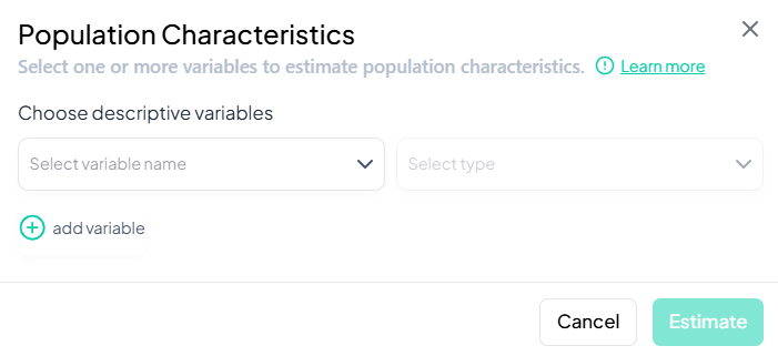
1. Population Characteristics

Purpose and Use Cases

• Describe sample demographics: age, sex, education
• Summarize categorical distributions: frequency and percentage
• Generate cohort profiles for reports or publications

Interface Walkthrough

1. Click Estimate > Population Characteristics.

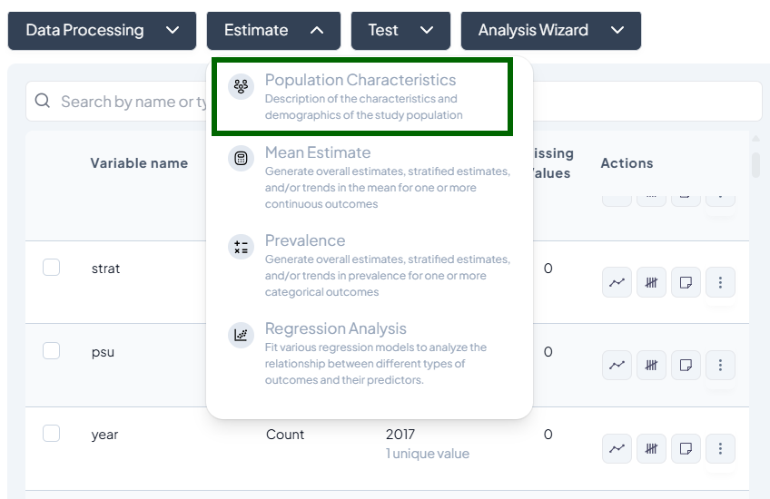
2. A modal appears: “Select one or more variables to estimate population characteristics.”
3. Contains:
   • Variable dropdown: list of categorical or continuous variables
   • Type dropdown: auto-detected (Continuous / Categorical)
   • Add variable button (+)

Step-by-Step Guide

1. Select Variables

   • Click the first dropdown and pick a variable (e.g., 'sex').
   • Ensure the detected type matches your intent (use Respecify in Data Processing if not).
   • Click + add variable to include more (e.g., 'age_group', 'education').

2. Define Population (optional)

   • By default, uses the entire dataset.
   • To subset: click Subset and build a filter (e.g., 'age ≥ 18').
   • Confirm the live record count.

3. Customize Display

   • Toggle Show missing values.
   • Choose Percent format (row vs. column).

4. Estimate

   • Click Estimate.
   • View table of counts and percentages.

   

Customization Options

• Row/Column percentages
• Suppress cells with low n (<5)
• Apply weights: check “Compute weighted counts” to use a weight variable

Output Interpretation

• Table: variable by category, N, %
• Metadata: sample size, subset filter, weight info
• Download: CSV, Excel

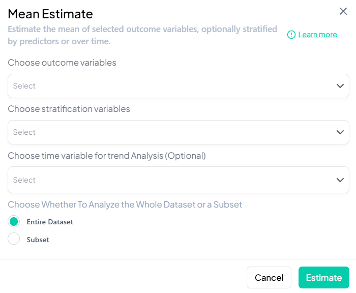
2. Mean Estimate

Purpose and Use Cases

• Compute central tendency (mean, median)
• Compare group means across strata or over time
• Trend analysis: show how means evolve

Interface Walkthrough

1. Click Estimate > Mean Estimate.
2. Modal fields:

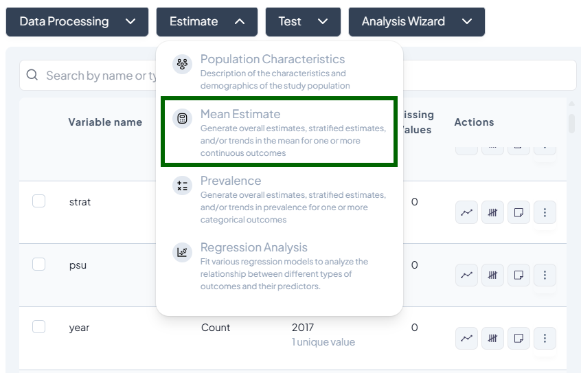
• Choose outcome variables (continuous)
• Choose stratification variables (categorical)
• Time variable for trend (date or numeric)
• Dataset scope: Entire vs. Subset

Step-by-Step Guide

1. Select Outcome

   • Pick one or multiple continuous variables (e.g., wt, height).

2. Select Stratifier (optional)

   • Add a grouping variable (e.g., 'sex').

3. Time Analysis (optional)

   • Choose a time variable (e.g., 'year') to display line charts.

4. Define Subset (optional)

   • Switch to Subset, specify filters, confirm N.

5. Advanced Settings

   • CI type: 95% normal vs. bootstrap
   • Precision cutoff: max coefficient of variation
   • Include missing-value summary

6. Estimate

   • Click Estimate to produce:

     • Table: mean, SD, CI
     • Chart: bar or line (if time included)

     

Customization Options

• Decimal precision for means
• CI display: bars on chart, table columns
• Overlay groups on time trends
• Apply survey weights if configured

Output Interpretation

• Table: rows per group (or overall), mean ± SD, CI bounds
• Chart: error bars indicate CI
• Export: PNG, SVG, CSV

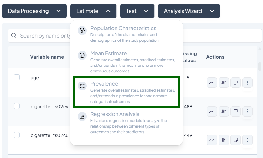
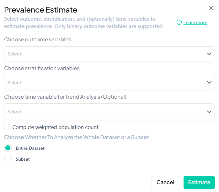
3. Prevalence

Purpose and Use Cases

• Estimate proportion of a binary outcome (e.g., disease = Yes)
• Stratify prevalence by demographics or time
• Assess change in prevalence trends

Interface Walkthrough

1. Click Estimate > Prevalence.

2. Modal includes:
   • Outcome variable (binary)
   • Stratification (categorical)
   • Time variable (optional)
   • Compute weighted population count checkbox
   • Whole vs. subset selector

Step-by-Step Guide

1. Select Binary Outcome (e.g., 'smoker_yes_no').

2. Add Stratifiers (e.g., 'sex', 'region').

3. Time Trend (optional): choose 'year' or date.

4. Weights

   • Tick Compute weighted population count to incorporate survey weights or calibration weights.

5. Subset (optional): define filters.

6. Estimate to get:

   • Table: N, prevalence%, CI
   • Chart: bar or line plot

   

Customization Options

• Precision thresholds for suppressing unstable estimates
• Alternate CI methods (Wilson, Agresti–Coull)
• Toggle denominator (unweighted vs. weighted)

Output Interpretation

• Table: prevalence %, CI, N per cell
• Chart: error bars, group comparisons
• Download: formats as above

4. Regression Analysis

Purpose and Use Cases

• Explore relationships between predictors and outcomes
• Predict outcomes from covariates
• Adjust for confounders in observational data

Supported Models

• Linear Regression
• Binary Logistic Regression
• Multinomial Logistic Regression
• Ordinal Logistic Regression
• Poisson Regression
• Negative Binomial Regression
• Probit Analysis

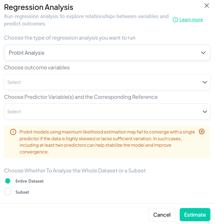
Interface Walkthrough

1. Click Estimate > Regression Analysis.

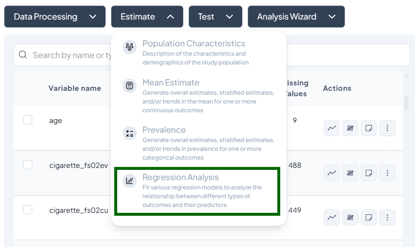
2. Modal: “Choose the type of regression analysis you want to run.”
3. Dropdown lists all supported models.

Step-by-Step Guide

1. Select Model Type (e.g., Binary Logistic).

2. Specify Variables

   • Outcome: continuous or categorical per model requirements.
   • Predictors: add one or more independent variables.
   • Covariates: optional adjustment set.
   • Stratification/Clustering: for complex survey designs.

3. Model Settings

   • Link function options (e.g., logit vs. probit).
   • Interaction terms: add via X * Z syntax.
   • Model fit criteria: AIC, BIC toggle.

4. Define Population (entire or subset).

5. Weights: apply calibration or survey weights.

6. Estimate

   • Click Estimate to run model.
   • After computation, view:
     • Coefficient table: estimates, SE, p-values, CI
     • Goodness of fit (R²/AUC)
     • Diagnostics plots (residuals, ROC curve)

Model-Specific Settings

• Linear: specify robust SE, cluster adjustment
• Logistic/Poisson: choose link, exposure offset (Poisson)
• Multinomial/Ordinal: reference category, parallel lines test

Output Interpretation

• Table: clear labeling of predictor effects
• Chart: forest plot of ORs/coefficients
• Diagnostics: clickable tabs, exportable charts

Pushing Outputs to Manuscript

All Estimate modules include a Push to Manuscript menu:

• Table only: inserts formatted table with title and footnotes
• Figure only: embeds chart with caption
• Table + Figure: both elements together
• Custom text: edit or add narrative around the output

How to use:

1. After running an analysis, click the ••• menu on the result.
2. Choose the push option.
3. In the manuscript pane, adjust the generated text if needed.
4. Save or export your document.

Test

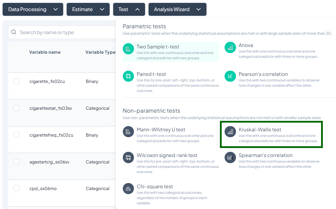
Use the Test subsection to perform hypothesis tests on your data, including parametric and nonparametric methods. Each test runs via a unified modal interface, letting you choose variables, define subsets, and view results as tables and charts.

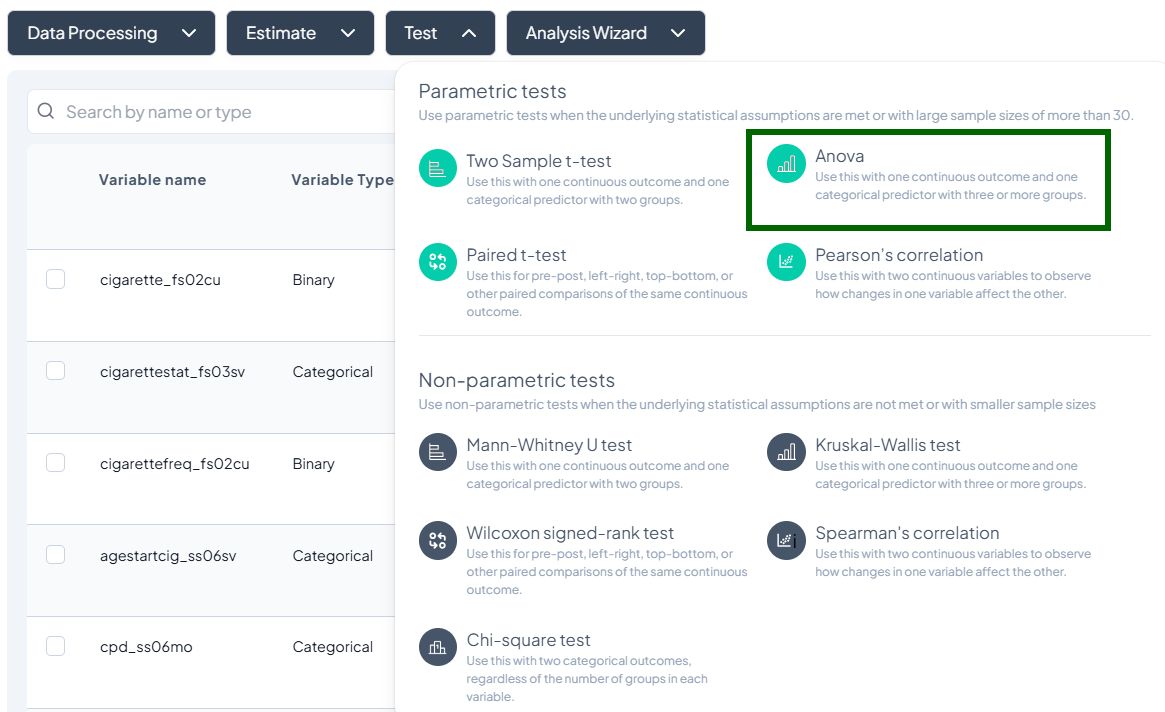
Accessing the Test Subsection

1. Click Test, a dropdown displays available tests, grouped by type:
   • Parametric tests (assume normality, large N)
   • Nonparametric tests (fewer assumptions, small samples)
2. Scroll or search to select your desired test.

Parametric Tests

1. Two-Sample t-Test

Purpose: Compare the means of a continuous outcome between two independent groups.

Assumptions:

• Outcome is approximately normally distributed within each group.
• Variances are equal (or use Welch’s correction).
• Observations independent.

Use Cases: Comparing blood pressure between treatment vs. control.

Step-by-Step:

1. Launch the Test modal: Test → Two-Sample t-Test.

2. Choose Outcome Variable: select a continuous variable (e.g., weight).
3. Choose Grouping Variable: select a categorical variable with exactly two levels (e.g., gender).
4. Subset (optional): switch to Subset dataset and define filters.
5. Options:
   • Toggle Assume equal variances (unchecked uses Welch’s t-test).
   • Include missing values if desired.
6. Click Test.

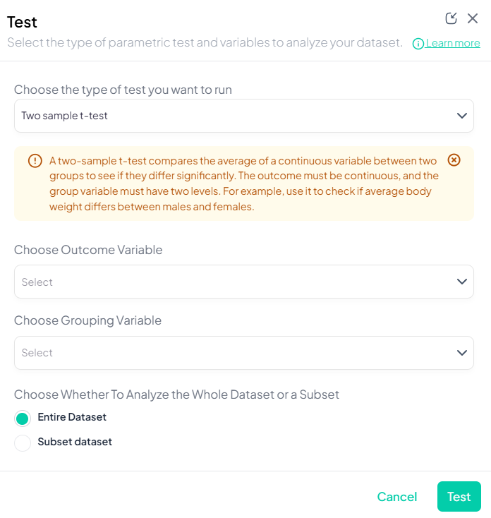
Output: table with group means, difference, t-statistic, df, two-sided p-value, CI for mean difference; boxplot by group.

2. One-Way ANOVA

Purpose: Test difference in means across three or more independent groups.

Assumptions:

• Normally distributed residuals.
• Homogeneity of variances.
• Independent observations.

Use Cases: Comparing mean test scores across multiple schools.

Step-by-Step:

1. Test → ANOVA.

2. Outcome Variable: select continuous measure.
3. Grouping Variable: select categorical with ≥3 levels.
4. Post-hoc options: Tukey’s HSD toggle (if desired).
5. Subset and weights as applicable.
6. Click Test.

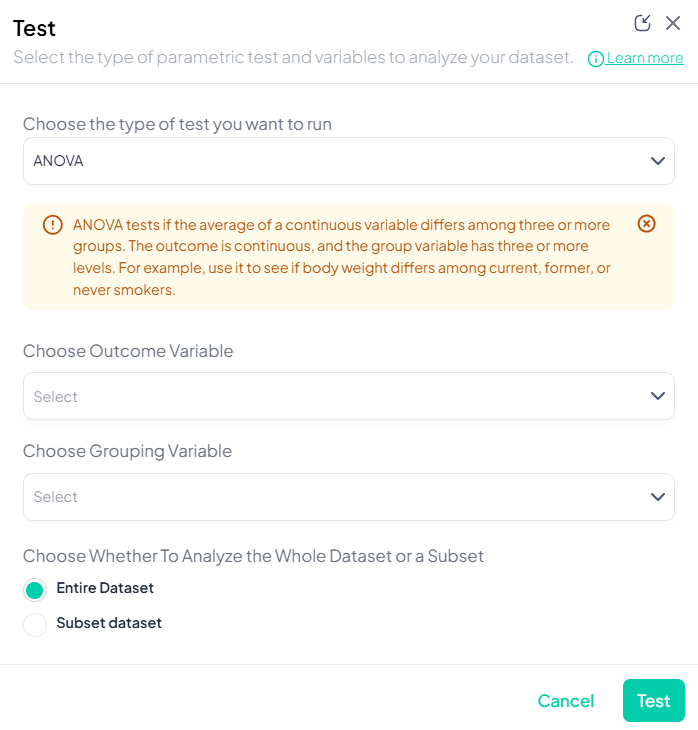
Output: ANOVA table (F, df, p), group means; optional pairwise comparisons chart.

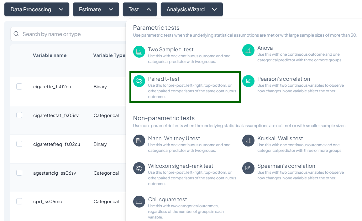
3. Paired t-Test

Purpose: Compare means of a continuous outcome measured twice on the same subjects.

Assumptions:

• Differences are normally distributed.
• Paired observations.

Use Cases: Pre- vs. post-treatment measurements on the same patients.

Step-by-Step:

1. Test → Paired t-Test.

2. Choose First Measurement: continuous variable at time1.
3. Choose Second Measurement: continuous variable at time2.
4. Subset (optional) and include missing as needed.
5. Click Test.

Output: mean difference ± SD, t-statistic, df, p-value; histogram of paired differences.

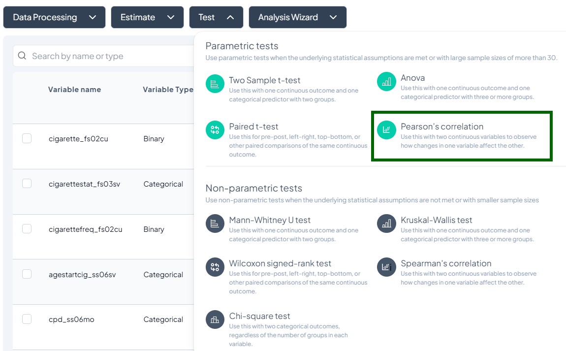
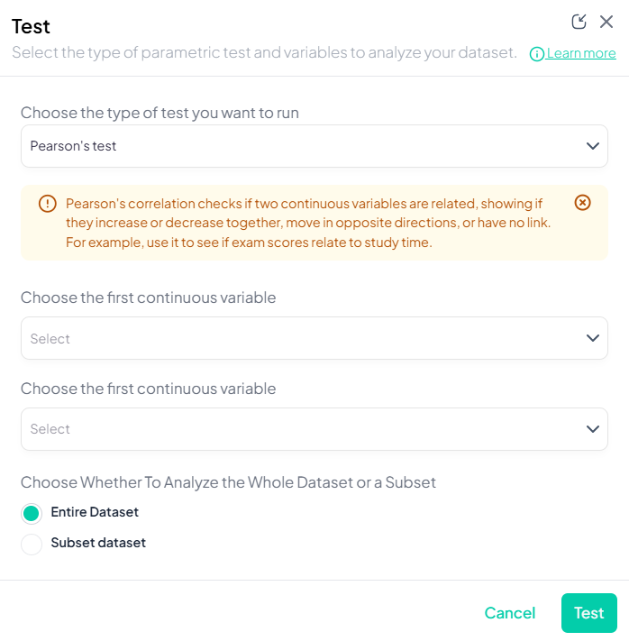
4. Pearson’s Correlation

Purpose: Measure linear association between two continuous variables.

Assumptions:

• Both variables normally distributed.
• Linear relationship.
• No extreme outliers.

Use Cases: Correlating height and weight.

Step-by-Step:

1. Test → Pearson’s correlation.

2. Select Variable X and Variable Y (both continuous).
3. Subset if needed.
4. Click Test.

Output: correlation coefficient (r), p-value, sample size; scatterplot with regression line.

Nonparametric Tests

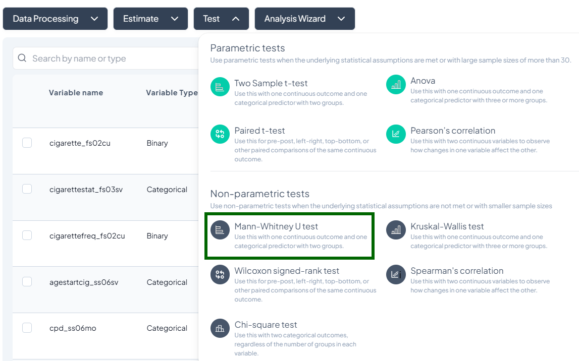
1. Mann–Whitney U Test

Purpose: Compare distributions of a continuous or ordinal outcome between two independent groups without assuming normality.

Assumptions:

• Independent samples.
• Ordinal or continuous data.

Use Cases: Comparing pain scores (ordinal) by treatment group.

Step-by-Step:

1. Mann–Whitney U Test.

2. Outcome Variable: continuous/ordinal.
3. Grouping Variable: binary categorical.
4. Include missing values (optional).
5. Subset as required.
6. Click Test.

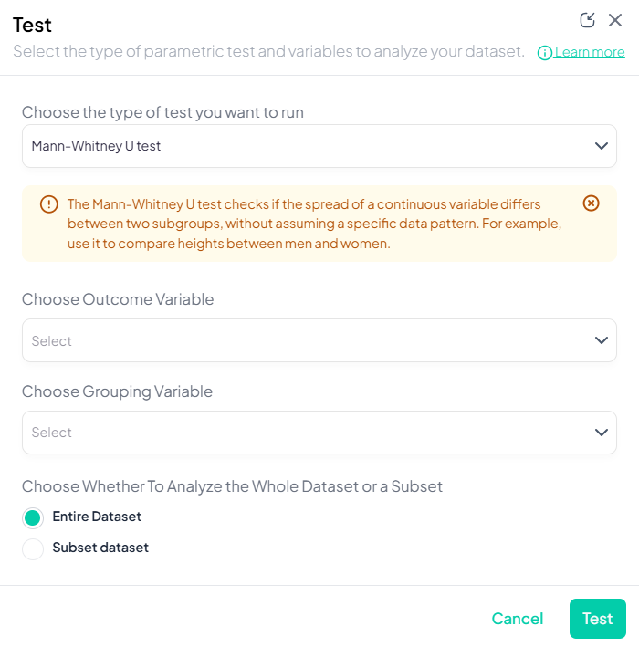
Output: U statistic, z-score, p-value; boxplots or violin plots by group.

2. Kruskal–Wallis Test

Purpose: Compare distributions across three or more groups without normality assumptions.

Assumptions:

• Independent groups.
• Ordinal/continuous outcome.

Use Cases: Comparing median incomes across regions.

Step-by-Step:

1. Test → Kruskal–Wallis Test.

2. Outcome Variable: continuous/ordinal.
3. Grouping Variable: categorical with ≥3 groups.
4. Subset optional.
5. Click Test.

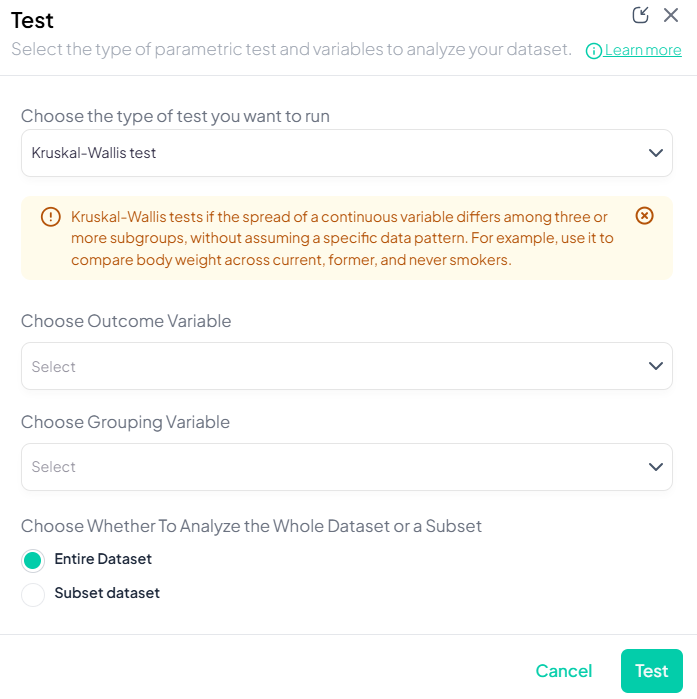
Output: H statistic, df, p-value; boxplots by group; post-hoc Dunn’s test option.

3. Wilcoxon Signed-Rank Test

Purpose: Compare paired differences for ordinal or continuous data without normality assumption.

Assumptions:

• Paired observations.
• Differences symmetrically distributed.

Use Cases: Pre/post Likert-scale survey on same participants.

Step-by-Step:

1. Test → Wilcoxon Signed-Rank Test.

2. Select Pair 1 and Pair 2 variables.
3. Include ties handling (drop or mid-rank).
4. Subset if needed.
5. Click Test.

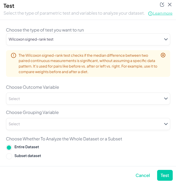
Output: V statistic, p-value; plot of difference ranks.

4. Spearman’s Correlation

Purpose: Assess monotonic association between two ordinal or continuous variables.

Assumptions:

• Variables at least ordinal.
• Monotonic relationship.

Use Cases: Rank-based correlation of survey items.

Step-by-Step:

1. Test → Spearman’s correlation.

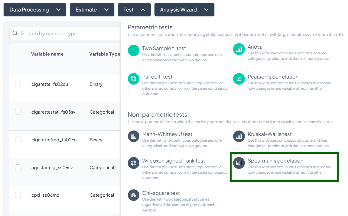
2. Variable X and Variable Y.
3. Subset if desired.
4. Click Test.

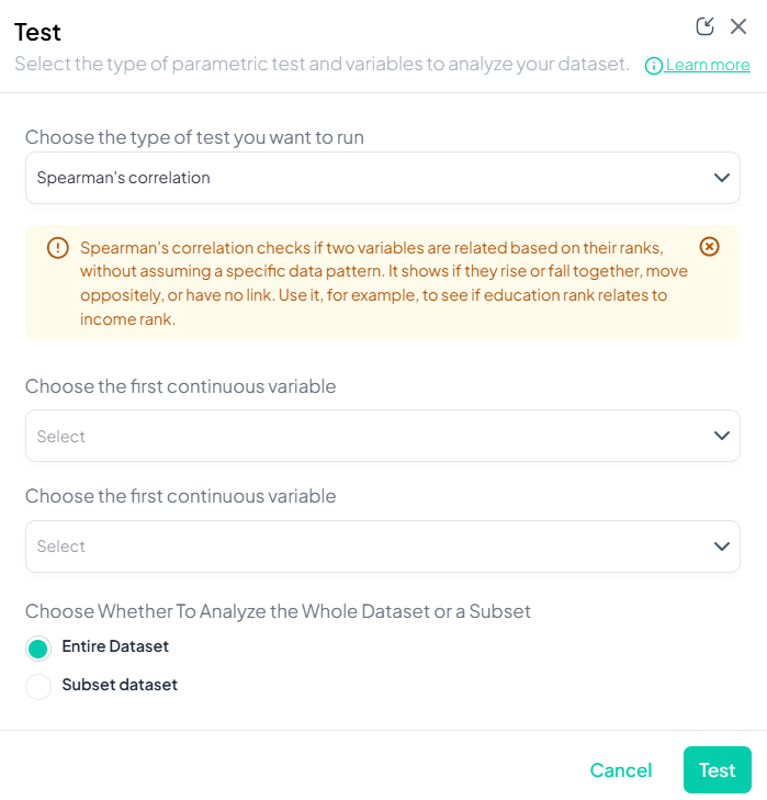
Output: Spearman’s ρ, p-value; scatterplot of ranks.

5. Chi-Square Test

Purpose: Test independence between two categorical variables.

Assumptions:

• Sufficient expected cell counts (>5 recommended).
• Observations independent.

Use Cases: Association between smoking status and disease presence.

Step-by-Step:

1. Test → Chi-Square Test.

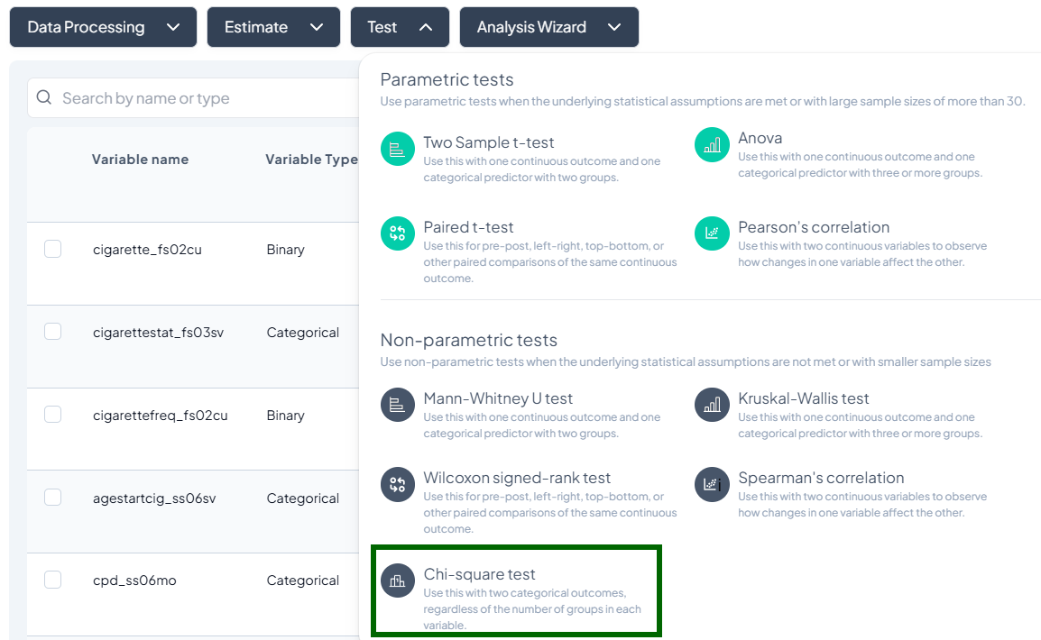
2. Select Row Variable and Column Variable (both categorical).
3. Subset dataset if needed.
4. Yates’ correction toggle for 2×2 tables.
5. Click Test.

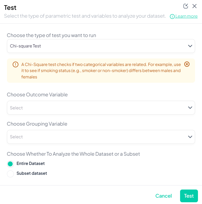
Output: χ² statistic, df, p-value; contingency table with counts and expected; mosaic or heatmap plot.

Unified Testing Workflow

All tests share a common modal structure:

1. Test Type dropdown (select your test).
2. Variable selectors tailored per test.
3. Options panel: missing-value inclusion, variance assumptions, post-hoc toggles.
4. Dataset scope: Entire vs. Subset (click to define filters).
5. Click Test to run.

Interpreting Outputs

• Result table: key statistics (test statistic, df, p-value, effect size).
• Visualization: contextual plots (boxplots, scatter, mosaic).
• Download/Share: export tables and charts, or push directly into manuscript.
• Metadata: record count, subset filters, options used.

Analysis Wizard Subsection

The Analysis Wizard offers AI-powered guidance to streamline your workflow: it recommends tables, selects appropriate tests, suggests regression models, and even generates research questions. This section details each Wizard feature—Analysis Suggester, Statistical Test Checker, Regression Analysis Checker, and Research Idea Suggester—with explanations, step-by-step instructions, and best practices.

Accessing the Analysis Wizard

1. Click Analysis Wizard.
2. Four options appear:
   • Analysis Suggester
   • Statistical Test Checker
   • Regression Analysis Checker
   • Research Idea Suggester
3. Select the desired tool.

1. Analysis Suggester

Purpose: AI-driven recommendations for tables and figures tailored to your dataset and specified variables.

Interface Elements

• Variable selectors:
  • Primary outcome with type dropdown
  • Secondary outcomes (1–10 slots, add via +)
  • Main predictor
  • Covariates
• Get suggestion buttons beside each section
• Preview Selected variables toggle
• Suggest Analysis action button
• Contextual notice at top indicating prior selections

Step-by-Step Guide

1. Click Analysis Wizard → Analysis Suggester.

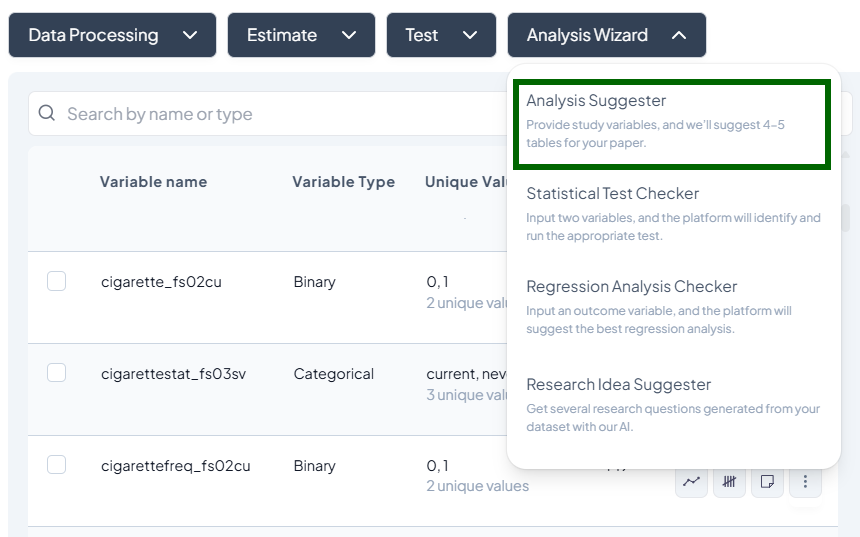
2. Select primary outcome:

   • Click first dropdown → choose variable.
   • Select its type (e.g., continuous, binary).
   • Optionally, click Get suggestion to auto-select based on data.

3. Add secondary outcomes:

   • Click + add variable, pick up to 10 variables.
   • Optionally, run Get suggestion.

4. Specify predictor and covariates similarly.

5. Preview:

   • Toggle Preview Selected variables to view data snapshots.

6. Suggest Analysis:

   • Click button; AI returns 4–5 recommended tables/figures with rationale.

   

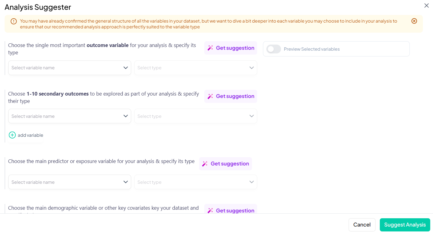
Tips & Customization

• Use Get suggestion to let AI surface variables with strongest signals.
• Adjust variable types via Data Processing first for accurate recommendations.
• Preview data to confirm sample sizes and distributions.

Output Interpretation

• Recommendations panel lists analyses (e.g., cross-tabs, trend lines).
• Each suggestion includes:
  • Description of table/figure
  • Variables involved
  • Next-step button to run directly

2. Statistical Test Checker

Purpose: Automatically identify and execute the correct hypothesis test given two variables and their data types.

Supported Tests

• Parametric: Two-sample t-test, Paired t-test, ANOVA, Pearson’s correlation
• Nonparametric: Mann–Whitney U, Wilcoxon signed-rank, Kruskal–Wallis, Spearman’s correlation, Chi-square

Step-by-Step Guide

1. Click Analysis Wizard → Statistical Test Checker.

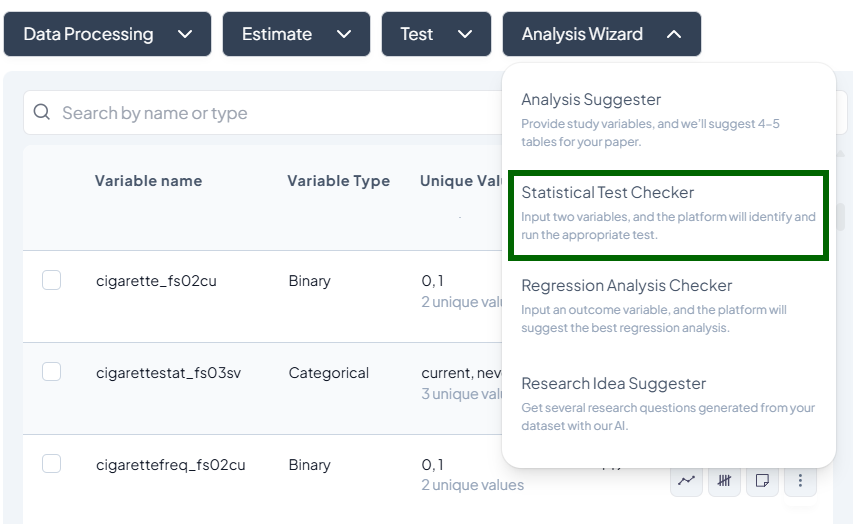
2. Select Variable 1:
   • Choose variable name and type dropdown (Continuous, Categorical, Ordinal).
3. Select Variable 2 similarly.
4. Preview (optional): toggle to see variable distributions.
5. Run: click Run; system selects appropriate test.

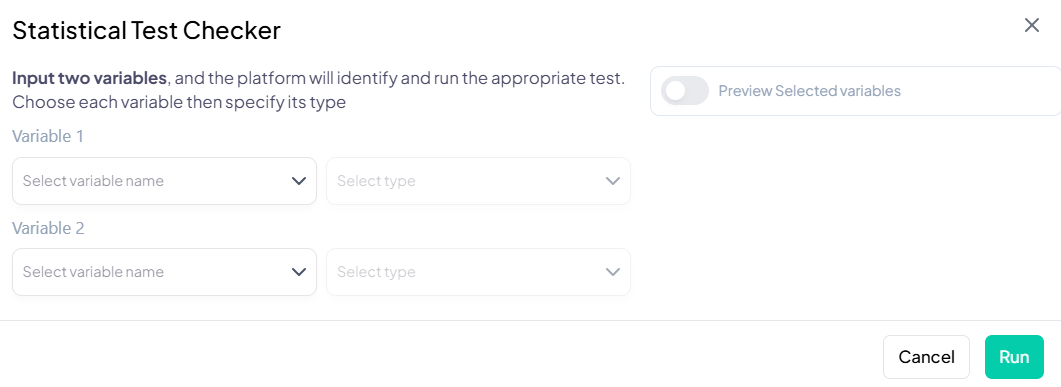
Test Selection Logic

• Variable types: match according to test assumptions (e.g., two continuous → Pearson or Spearman).
• Paired vs. independent: if both variables share ID or time context, suggests paired options.
• Group levels: categorical must have required number of levels (2 or ≥3).

Reviewing Results

• Output modal displays:
  • Test name and rationale (why selected)
  • Result table with statistic, p-value, effect size
  • Visualization (boxplot, scatter, contingency table)
• Options to push table/plot to manuscript or export.

3. Regression Analysis Checker

Purpose: Recommend and run the optimal regression model based on your outcome variable and its measurement context.

Supported Models

Linear, Logistic (binary, multinomial, ordinal), Poisson, Negative Binomial, Probit.

Step-by-Step Guide

1. Click Analysis Wizard → Regression Analysis Checker.

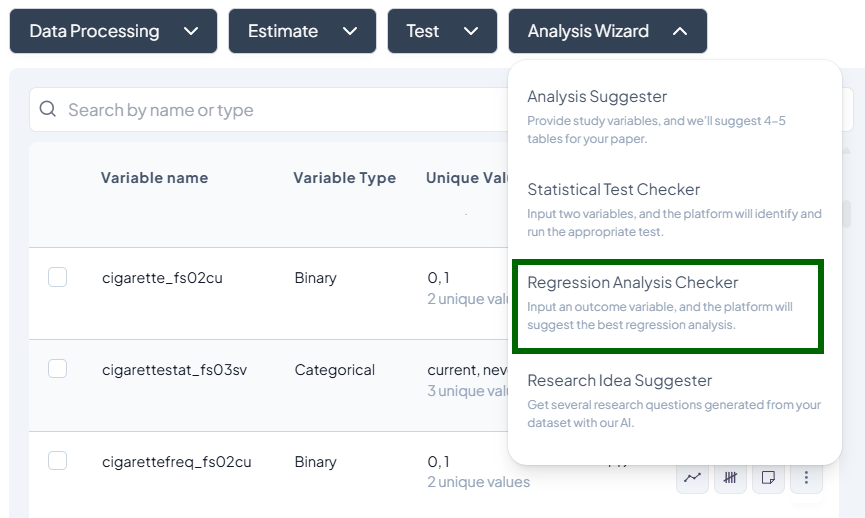
2. Select Outcome Variable:
   • Choose from dropdown; specify type (Continuous, Binary, Count, Ordinal).
3. Measurement frequency:
   • Use dropdown to indicate one-time vs. repeated measures.
4. Preview predictors if toggle enabled.
5. Run: click Run; AI recommends model(s).

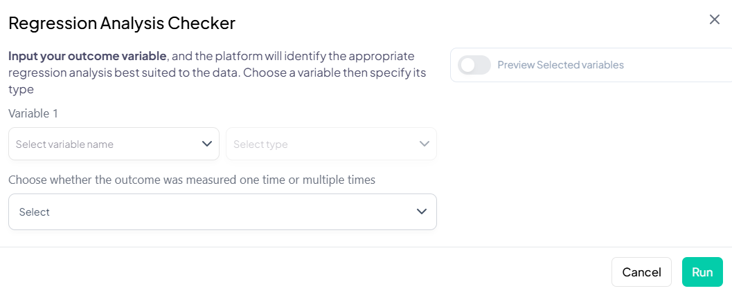
Model Recommendation Criteria

• Outcome type → linear vs. logistic vs. count model
• Repeated measures flag → mixed effects or GEE (if supported)
• Distributional checks on outcome (e.g., skewness triggers NB over Poisson)

Next Steps

• Review suggested model with parameter list (predictors default to covariates from wizard).
• Customize: add/remove predictors, interaction terms, clustering.
• Estimate and inspect outputs as per Regression module.

4. Research Idea Suggester

Purpose: Generate AI-crafted research questions and hypotheses grounded in your dataset’s variables and structure.

Step-by-Step Guide

1. Click Analysis Wizard → Research Idea Suggester.

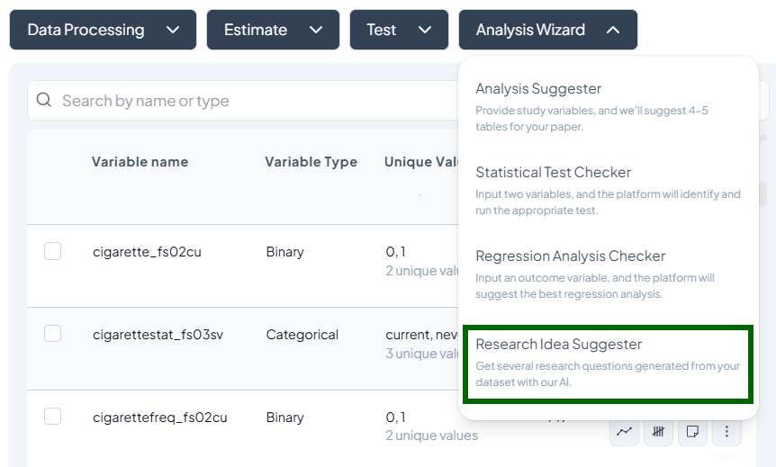
2. Loading screen: platform analyzes variable metadata.
3. View Suggestions:
   • Up to 10 questions appear in list form.
4. Regenerate: click to get a fresh set of ideas.
5. Copy or export the questions for your study proposal.

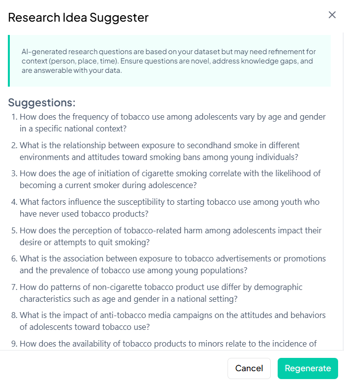
AI Guidance & Limitations

• Questions are based on variable names and types; context (population, setting) must be refined.
• Use as brainstorming starting points, not final hypotheses.

Refining Questions

• Tailor by injecting dataset metadata (year, region).
• Verify novelty against literature.
• Ensure feasibility given sample size and variable distribution.

Common Workflow & Best Practices

• Clean and respecify your variables in Data Processing before using any Wizard tool to ensure correct type detection.
• Preview data via toggles to confirm sample sizes, distributions, and missingness.
• Iterate suggestions: use AI features to speed selection, then customize parameters manually.
• Push results to manuscript draft directly from all Wizard outputs to maintain reproducibility.
• Validate AI recommendations against statistical assumptions and domain knowledge.

Conclusion

The Chisquares Data Analysis module is a powerful tool for transforming survey responses into actionable insights. With an intuitive design and robust filtering options, users can efficiently analyze their data and make informed decisions.

For further assistance, access the Help? button in the lower-left for extended support.